rpact and RPACT Cloud in Practical Use
November 13, 2025
rpact and RPACT Cloud in Practical Use

Example illustrating the package concept
Usage inspired by the typical workflow in trial design and conduct:
- Everything is starting with a design, e.g.:
design <- getDesignGroupSequential() - Find the optimal design parameters:
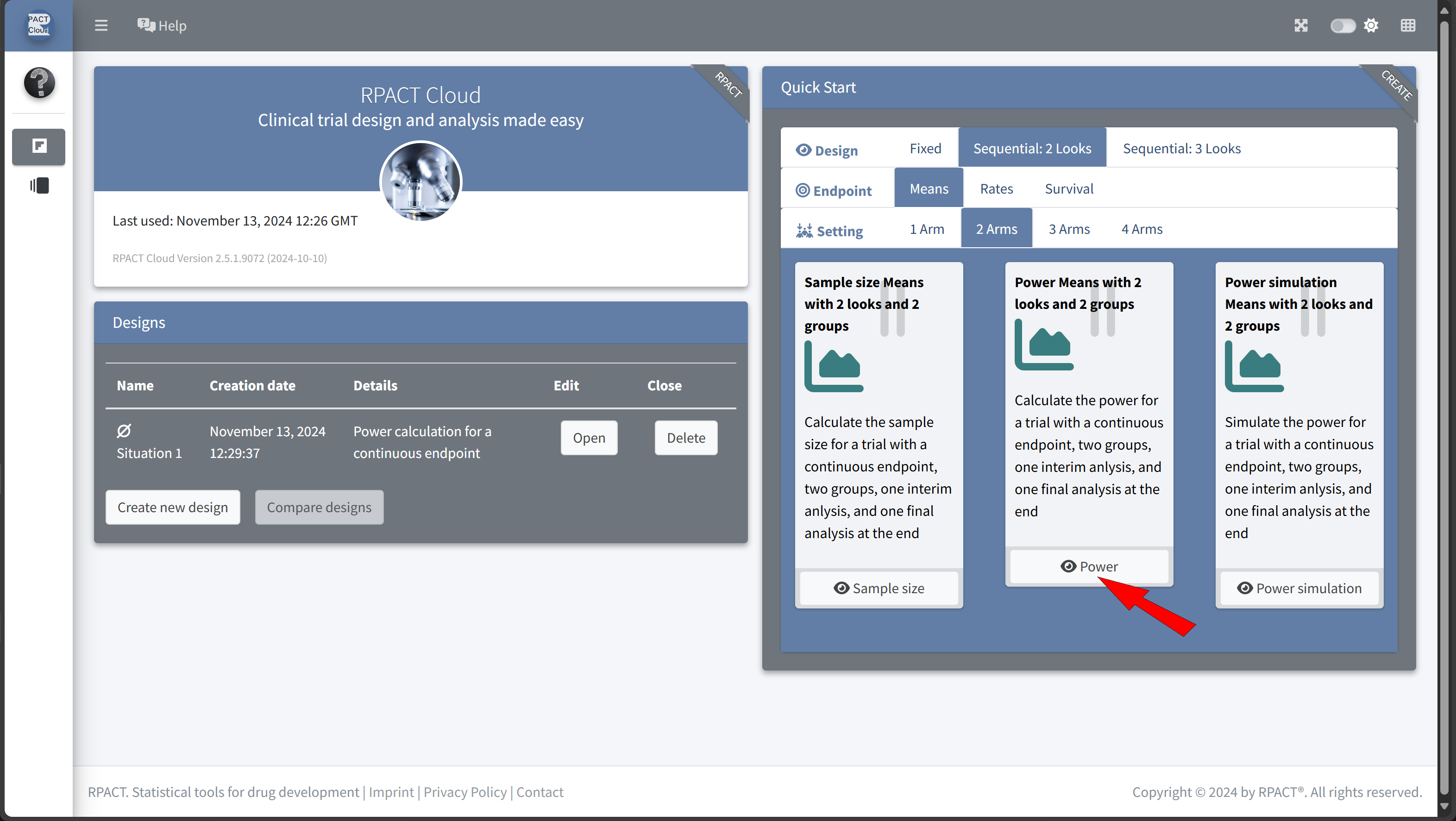
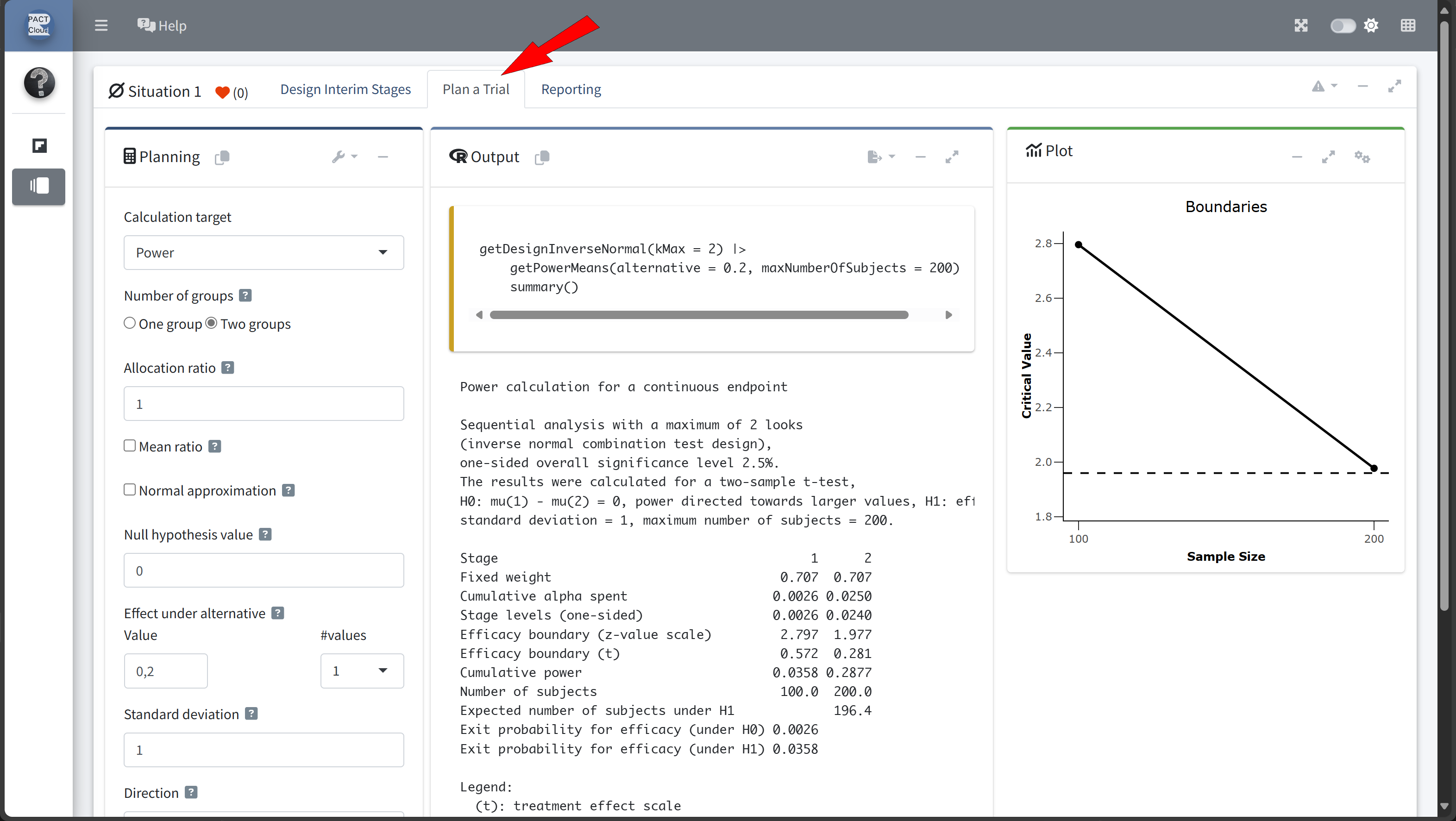
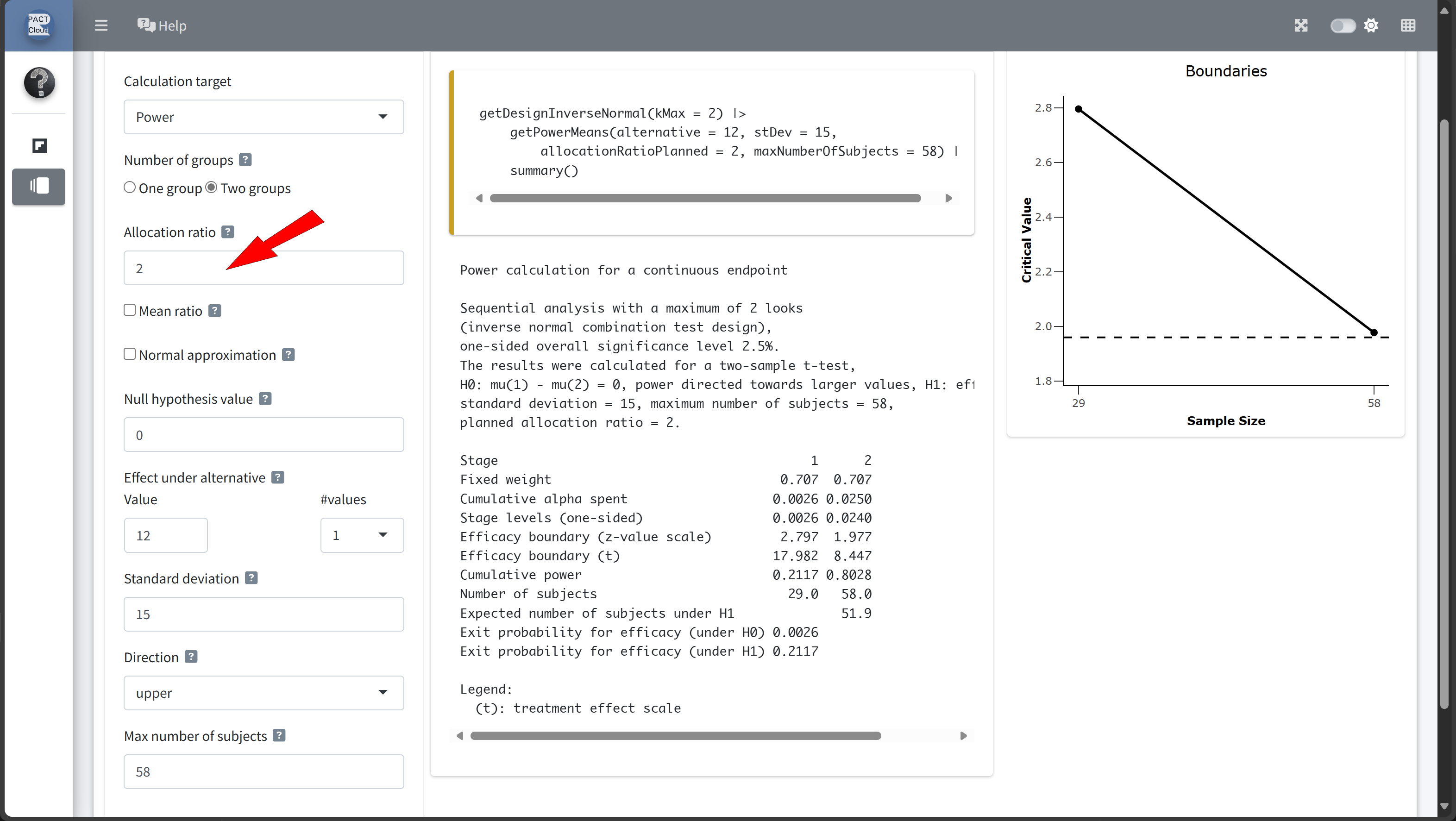
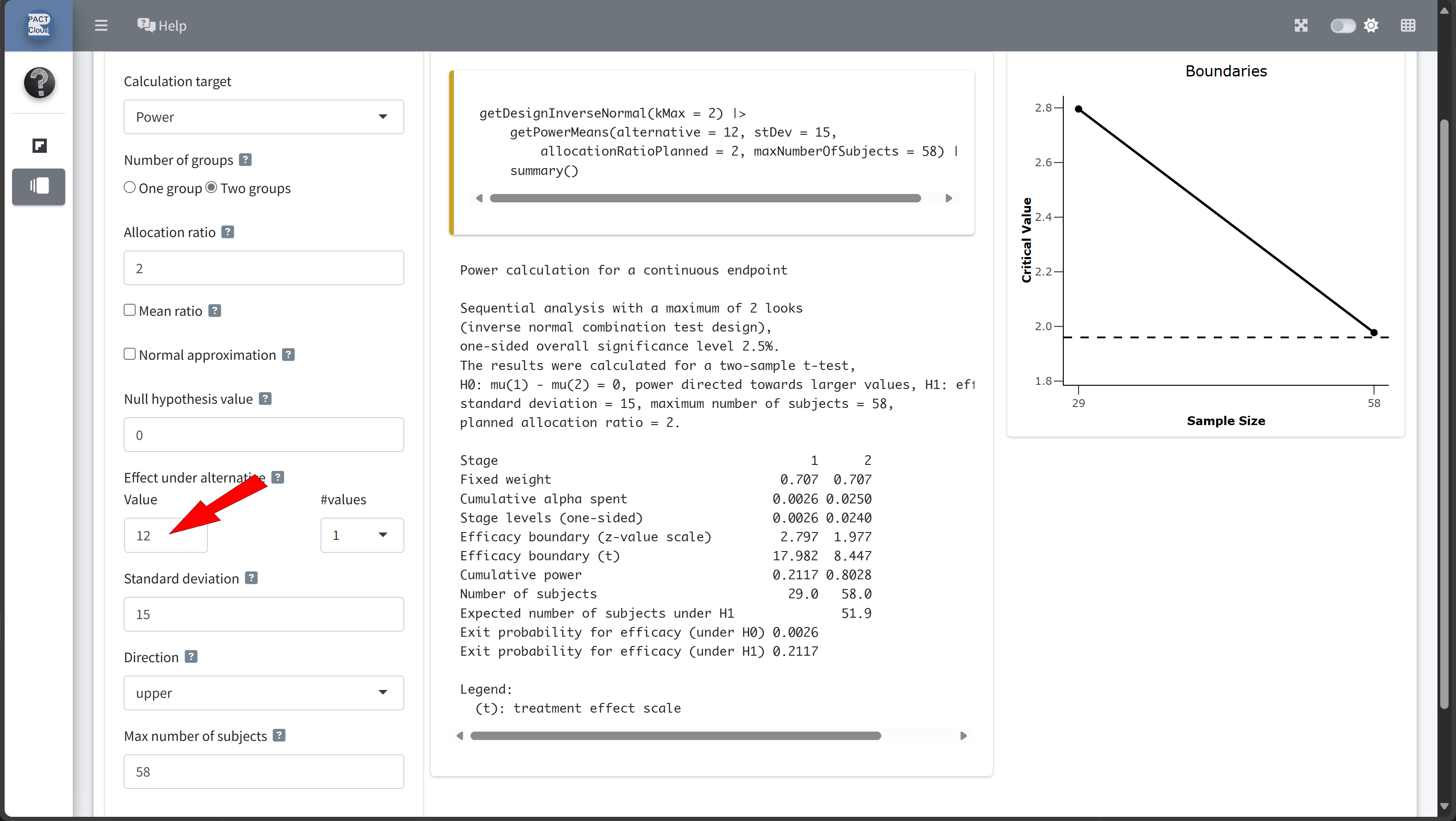
R / rpact / RPACT Cloud - Calculate the required sample size and power, e.g.:
getSampleSizeMeans(),getPowerMeans() - Collect your data, import it into R and create an rpact dataset:
data <- getDataset() - Analyze your data:
getAnalysisResults(design, data)
Example: Planning and Conducting a Clinical Study Using R and rpact
- In this fictive example, we will illustrate the planning and conduct of a clinical trial to assess the effectiveness of a new antihypertensive therapy.
- Each step will be demonstrated using R, primarily with the rpact package and RPACT Cloud.
- Additional R packages may be used as needed.
Study Design
Objective: To evaluate the effect of a new antihypertensive therapy
(compared to a placebo) in patients with hypertension.
Endpoints and Assumptions:
- Endpoint: Continuous endpoint (blood pressure reduction).
- Comparison Groups: New Treatment vs. Placebo.
- Statistical Parameters:
- One-sided test with \(\alpha\) = 0.025.
- Power = 80%.
Initial Assumptions and Parameter Estimation
Assumptions:
- Patients in this study suffer from high blood pressure (grade 2 hypertension), often around 150 mmHg (systolic).
- The objective is to significantly reduce blood pressure in the treatment group, while no substantial reduction is expected in the placebo group.
Expected Values:
- Expected reduction in systolic blood pressure:
12 mmHg. - Difference of baseline values and values after treatment:
Standard deviation of 15 mmHg.
Step 1: Sample Size Calculation
rpact: we will calculate the required sample size to achieve a power of 80% for detecting a 12 mmHg reduction in systolic blood pressure in the treatment group.
# Load the rpact package
library(rpact)

# Define the design parameters for sample size calculation
design <- getDesignGroupSequential(
    kMax  = 1,     # Only one analysis (classic fixed design)
    alpha = 0.025, # Significance level
    beta  = 0.20,  # 80% power
    sided = 1      # One-sided test
)

# Estimate sample size
sampleSizeResult <- design |>
    getSampleSizeMeans(
        groups = 2,       # Two groups: Treatment vs. Placebo
        alternative = 12, # Expected effect size
                          # (mean difference: 150 - 138 mmHg)
        stDev = 15        # Common standard deviation
)Sample size calculation for a continuous endpoint
Fixed sample analysis, one-sided significance level 2.5%, power 80%. The results were calculated for a two-sample t-test, H0: mu(1) - mu(2) = 0, H1: effect = 12, standard deviation = 15.
| Stage | Fixed |
|---|---|
| Stage level (one-sided) | 0.0250 |
| Efficacy boundary (z-value scale) | 1.960 |
| Efficacy boundary (t) | 8.438 |
| Number of subjects | 51.0 |
Legend:
- (t): treatment effect scale
Step 2: Calculating Power for the Study Design
Calculating power helps us:
- Verify the Assumptions: Ensure that the chosen sample size truly yields the expected 80% power, given random variations in the data.
- Explore Outcome Variability: Observing power across different situations can reveal potential inconsistencies in achieving the target power, especially with variations in standard deviation or effect size.
- Adjust Study Design: If the results show that power is consistently below the target, we might need to increase the sample size or reconsider assumptions.
Power Calculation Code
Using the rpact package, we can calculate the power of the study under the defined parameters. Here’s how:
# Define parameters based on initial assumptions
calculatedSampleSize <-
sampleSizeResult$numberOfSubjects |> ceiling()
powerResult <- design |>
getPowerMeans(
groups = 2, # Two groups: Treatment and Placebo
alternative = 12, # Expected effect size
# (mean difference: 150 - 138 mmHg)
stDev = 15, # Common standard deviation
maxNumberOfSubjects = calculatedSampleSize
)
# Print the summary of the the results
powerResult |> summary()Power calculation for a continuous endpoint
Fixed sample analysis, one-sided significance level 2.5%. The results were calculated for a two-sample t-test, H0: mu(1) - mu(2) = 0, power directed towards larger values, H1: effect = 12, standard deviation = 15, number of subjects = 52.
| Stage | Fixed |
|---|---|
| Stage level (one-sided) | 0.0250 |
| Efficacy boundary (z-value scale) | 1.960 |
| Efficacy boundary (t) | 8.356 |
| Power | 0.8075 |
| Number of subjects | 52.0 |
Legend:
- (t): treatment effect scale
- The results show that in 80.75% of the trials the test successfully detect a true difference between treatment and control group.
- Next steps: proceed with further setup and explore possible adjustments based on the outcomes.
Exploring Possible Adjustments Based on Power Calculation Outcomes
- Varying Effect Size: If the expected effect size of 12 mmHg is optimistic, we could calculate a scenario with a smaller effect size (e.g., 10 mmHg) to see how it affects the required sample size and power.
- Varying Standard Deviation: The assumed standard deviation of 15 mmHg might vary across patient groups. Increasing it to 16 or 17 mmHg would allow us to explore how higher variability impacts power and the required sample size.
Example Code for Possible Adjustments in R
Here’s R code to analyze the scenarios described above:
# Define scenarios for adjustments
scenarios <- list(
list(alternative = 10, stDev = 15), # 1: Reduced effect
list(alternative = 10, stDev = 14), # 2: Reduced effect + sd
list(alternative = 11, stDev = 15), # 3: Reduced effect
list(alternative = 11, stDev = 14), # 4: Reduced effect + sd
list(alternative = 12, stDev = 15), # 5: Base scenario
# with 12 mmHg effect
list(alternative = 13, stDev = 16), # 6: Incr. sd + effect
list(alternative = 13, stDev = 17), # 7: Incr. sd + effect
list(alternative = 12, stDev = 16), # 8: Increased sd
list(alternative = 12, stDev = 17) # 9: Increased sd
)
# Run calculations for each scenario
results <- scenarios |>
lapply(function(scenario) {
getPowerMeans(
design = design,
groups = 2,
alternative = scenario$alternative,
stDev = scenario$stDev,
maxNumberOfSubjects = 52
)
}
)
# Fetch only the power from the result objects
x <- sapply(results, function(result) {
result |> fetch("Overall reject")
})| alternative | stDev | power | |
|---|---|---|---|
| Szenario 1 | 10 | 15 | 0.6544534 |
| Szenario 2 | 10 | 14 | 0.7142007 |
| Szenario 3 | 11 | 15 | 0.7366421 |
| Szenario 4 | 11 | 14 | 0.7933714 |
| Szenario 5 | 12 | 15 | 0.8074858 |
| Szenario 6 | 13 | 16 | 0.8193392 |
| Szenario 7 | 13 | 17 | 0.7715373 |
| Szenario 8 | 12 | 16 | 0.7555122 |
| Szenario 9 | 12 | 17 | 0.7040188 |
Interpretation of Scenarios
- Base scenario (52 subjects, 12 mmHg effect, 15 mmHg SD): Verifying the original power (around 80.75%).
- Reduced effect size (10 mmHg effect): With a smaller effect size, the power to drop to 65.45%. This illustrates that the study is not very robust if the actual effect is smaller than expected.
- Increased standard deviation (17 mmHg SD): Increasing variability lowers the power to 70.4%, as greater variability results in less precise outcomes.
By exploring these adjustments, we gain insight into whether a larger sample or refined target parameters might be needed for a more reliable assessment of the drug’s efficacy.
Ethical Considerations: Exploring Scenarios with Larger Treatment Group
- Explore scenarios with unequal allocation ratios, assigning more participants to the treatment group than to the control group.
- This approach allows more patients the potential benefit of the new therapy while still maintaining a control group for reliable statistical comparison.
- The
allocationRatioPlannedargument inrpactenables us to specify these ratios.
Scenario Adjustments Using Unequal Allocation Ratios
Here are the new scenarios we will examine:
- Base scenario (1:1 allocation): Both groups (treatment and control) have equal numbers of participants.
- 2:1 allocation: For every 1 participant in the control group, 2 are assigned to the treatment group.
- 3:1 allocation: For every 1 participant in the control group, 3 are assigned to the treatment group.
Comparing Different Allocation Ratios
Using the rpact package, we can set up and calculate these scenarios with the allocationRatioPlanned parameter:
# Define the initial design
design <- getDesignGroupSequential(
kMax = 1,
alpha = 0.025,
beta = 0.2,
sided = 1
)
# Define scenarios for different allocation ratios
scenarios <- list(
list(allocationRatio = 1), # 1:1 allocation
list(allocationRatio = 2), # 2:1 allocation
list(allocationRatio = 3) # 3:1 allocation
)
# Run calculations for each scenario with specified allocation ratios
results <- scenarios |>
lapply(function(scenario) {
getPowerMeans(
design = design,
groups = 2,
alternative = 12,
stDev = 15,
maxNumberOfSubjects = 50,
allocationRatioPlanned = scenario$allocationRatio
)
}
)
# Fetch only the power from the result objects
x <- sapply(results, function(result) {
result |> fetch("Overall reject")
})| allocationRatio | power | |
|---|---|---|
| Szenario 1 | 1 | 0.7914502 |
| Szenario 2 | 2 | 0.7431284 |
| Szenario 3 | 3 | 0.6701351 |
Let’s assume that an 2:1 allocation shall be used.
Continuing with a Group-Sequential Design to Open Up the Opportunity for Early Stopping
Given the slight reduction in power observed with the 2:1 allocation ratio (Power = 74.31%), we can implement a group-sequential design with an interim analysis instead of simply increasing the sample size.
With this approach:
- Planned Interim Analysis:
- After enrolling a number yet to be determined participants, an interim analysis will be conducted.
- Potential Outcomes:
- If the treatment shows significant efficacy at the interim point, the study can be stopped early to avoid additional recruitment.
- If efficacy is not yet demonstrated, we proceed to the full planned sample size.
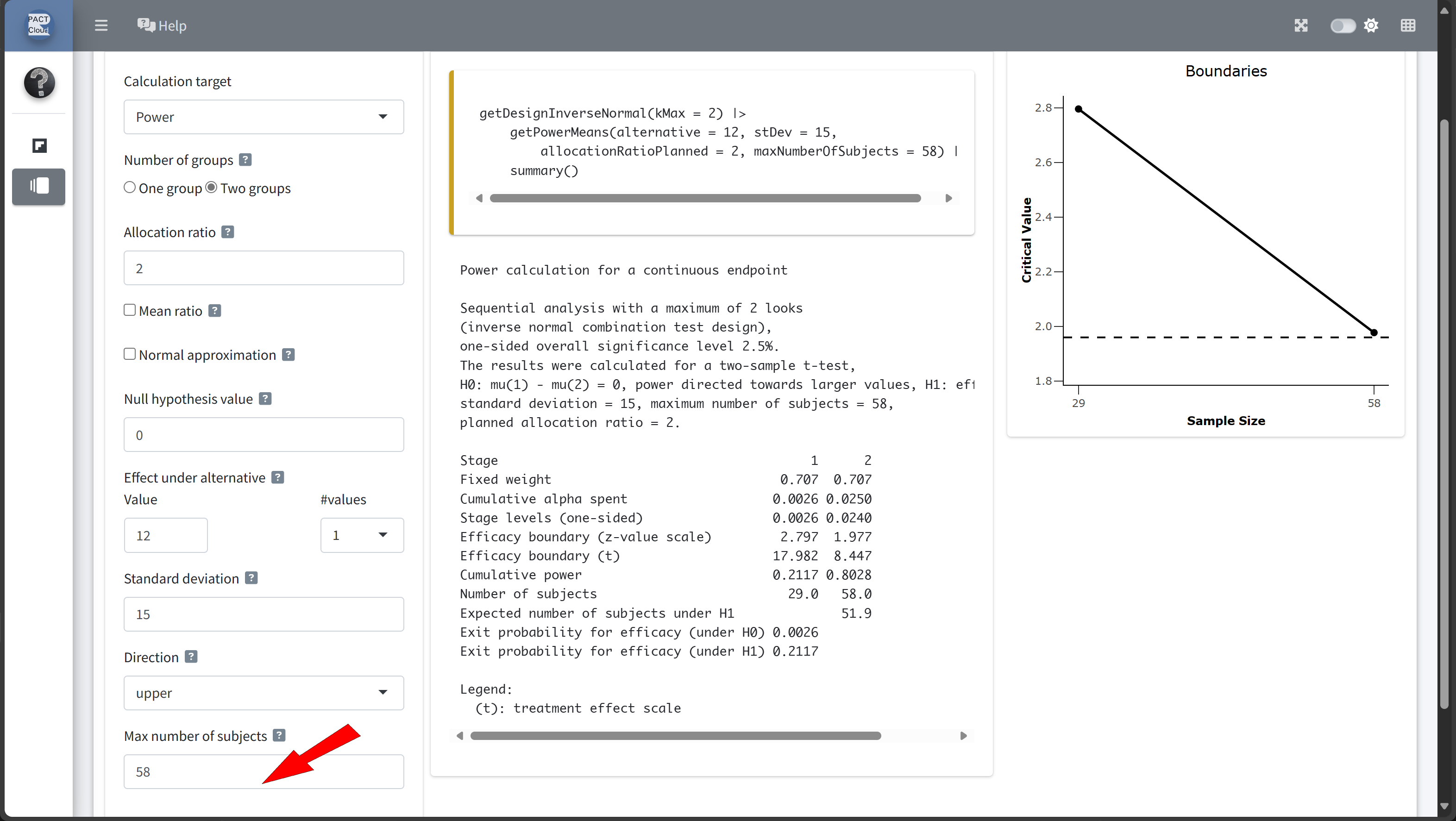
Step 1: Calculate the sample size for a fixed design
nFixed
58 We need numberOfSubjectsFixed for the subsequent power analysis.
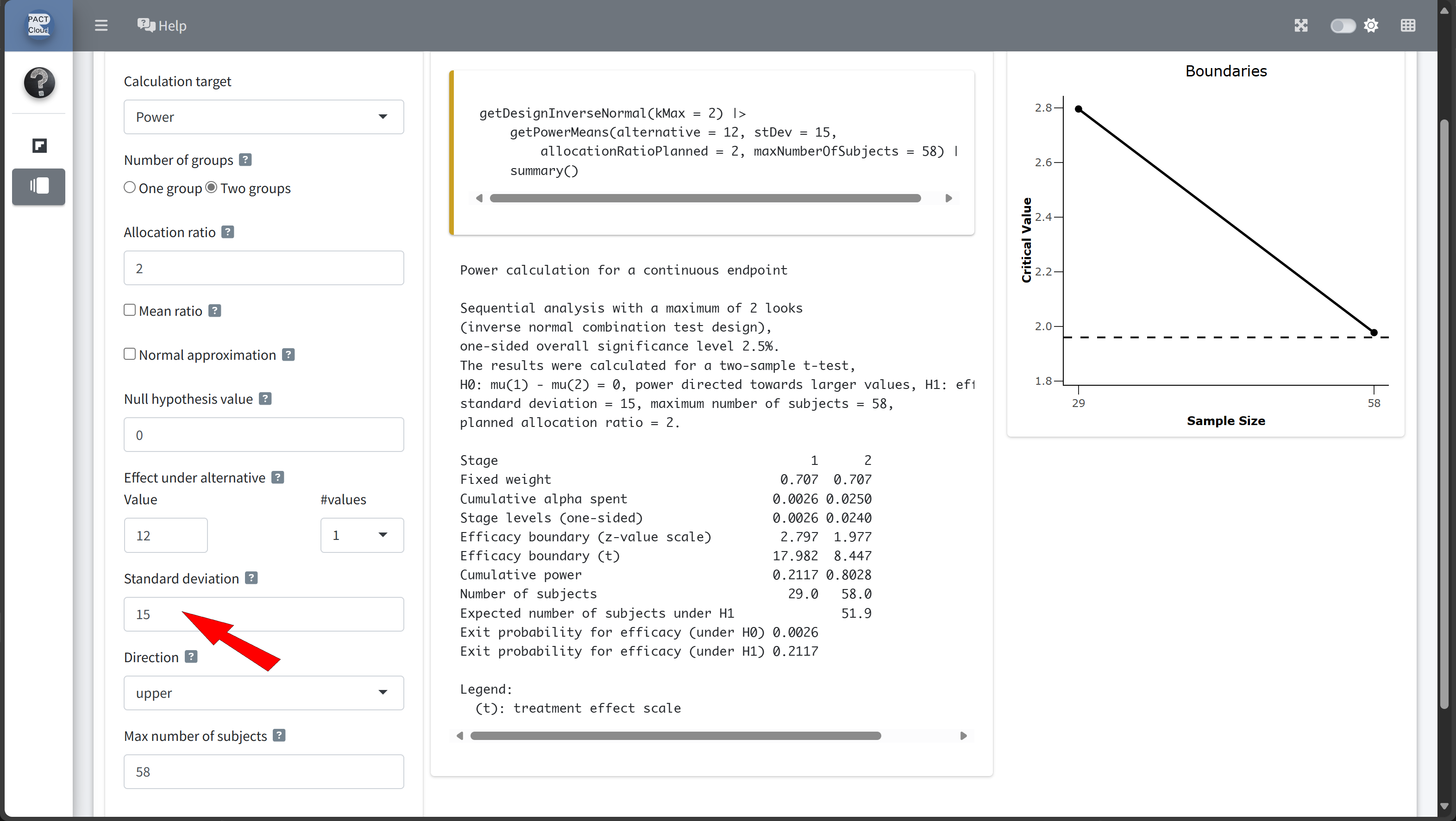
Step 2: Define the Group-Sequential Design with an Interim Analysis
- We’ll use
rpactto define a group-sequential design with two planned analyses. - The first analysis will occur after enrolling
nsubjects, with a final analysis if the study proceeds to the full sample. nshall be determined by exploring different information rates
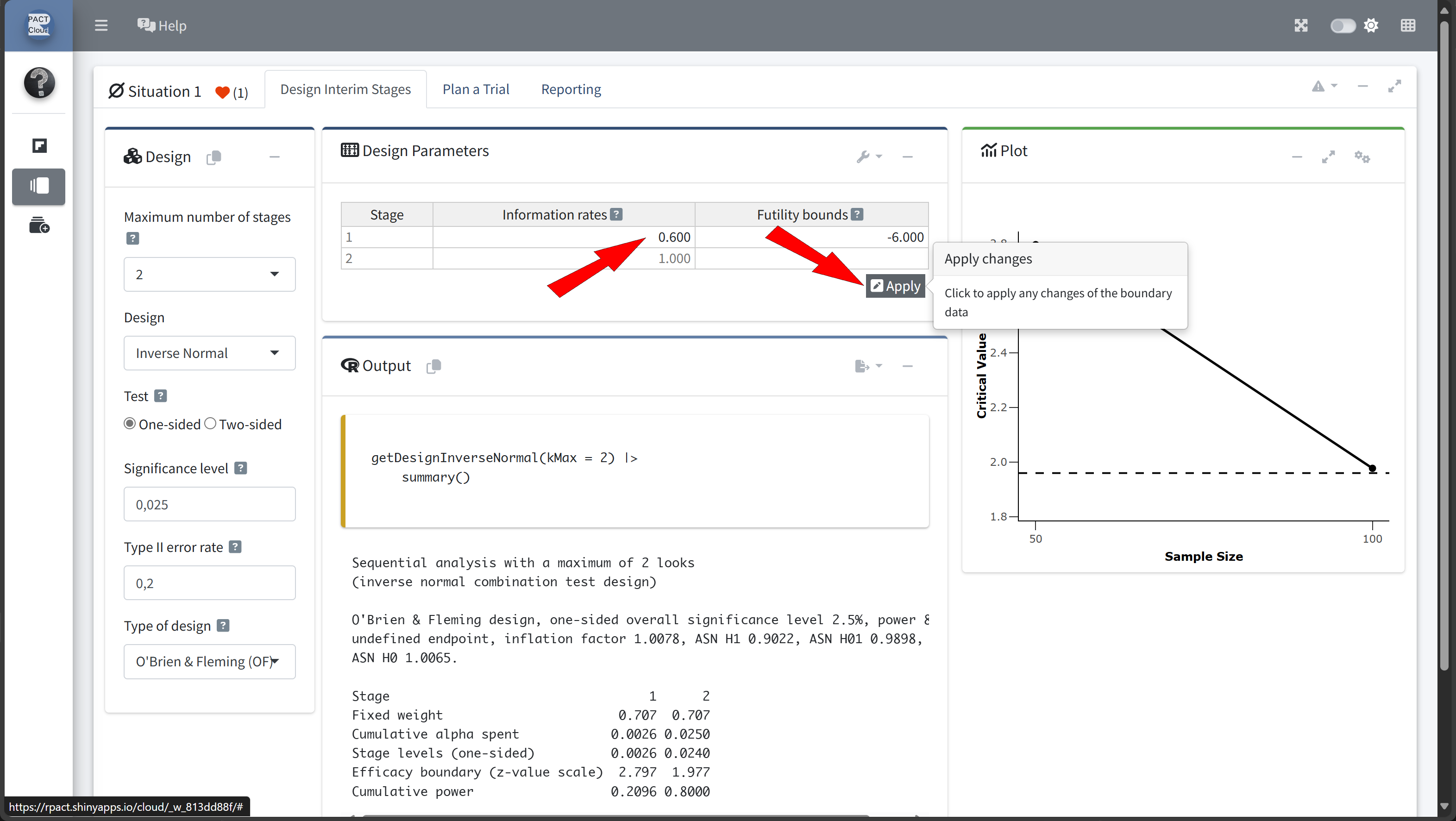
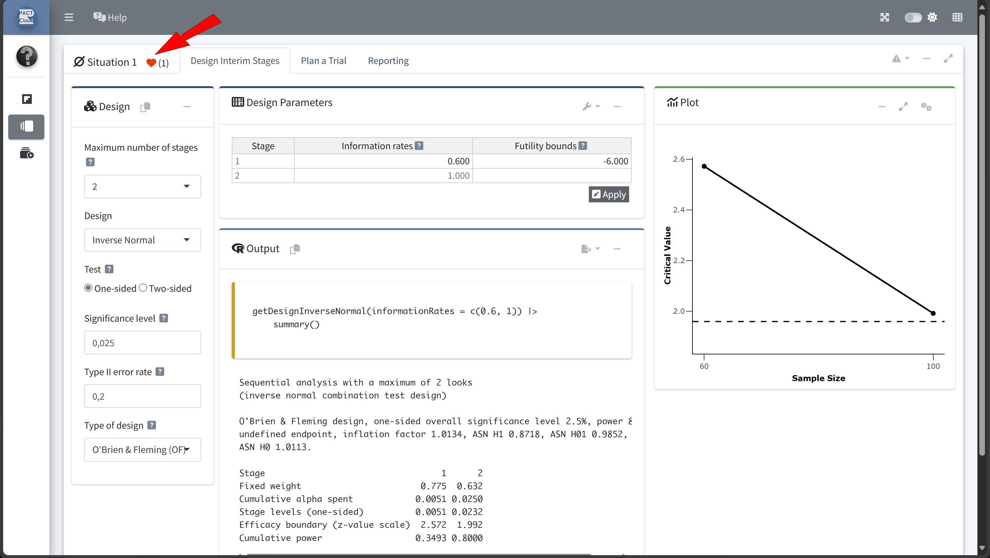
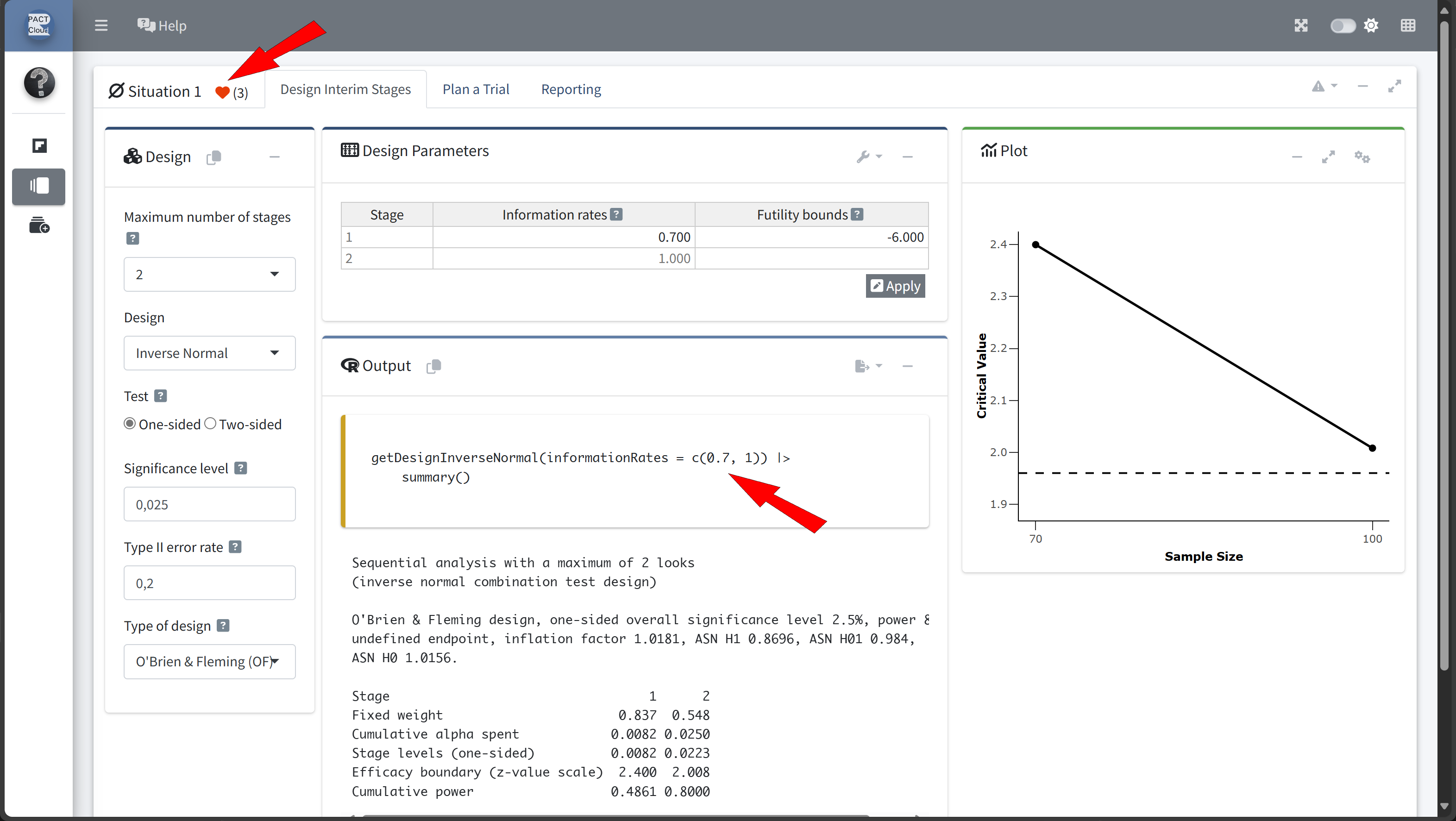
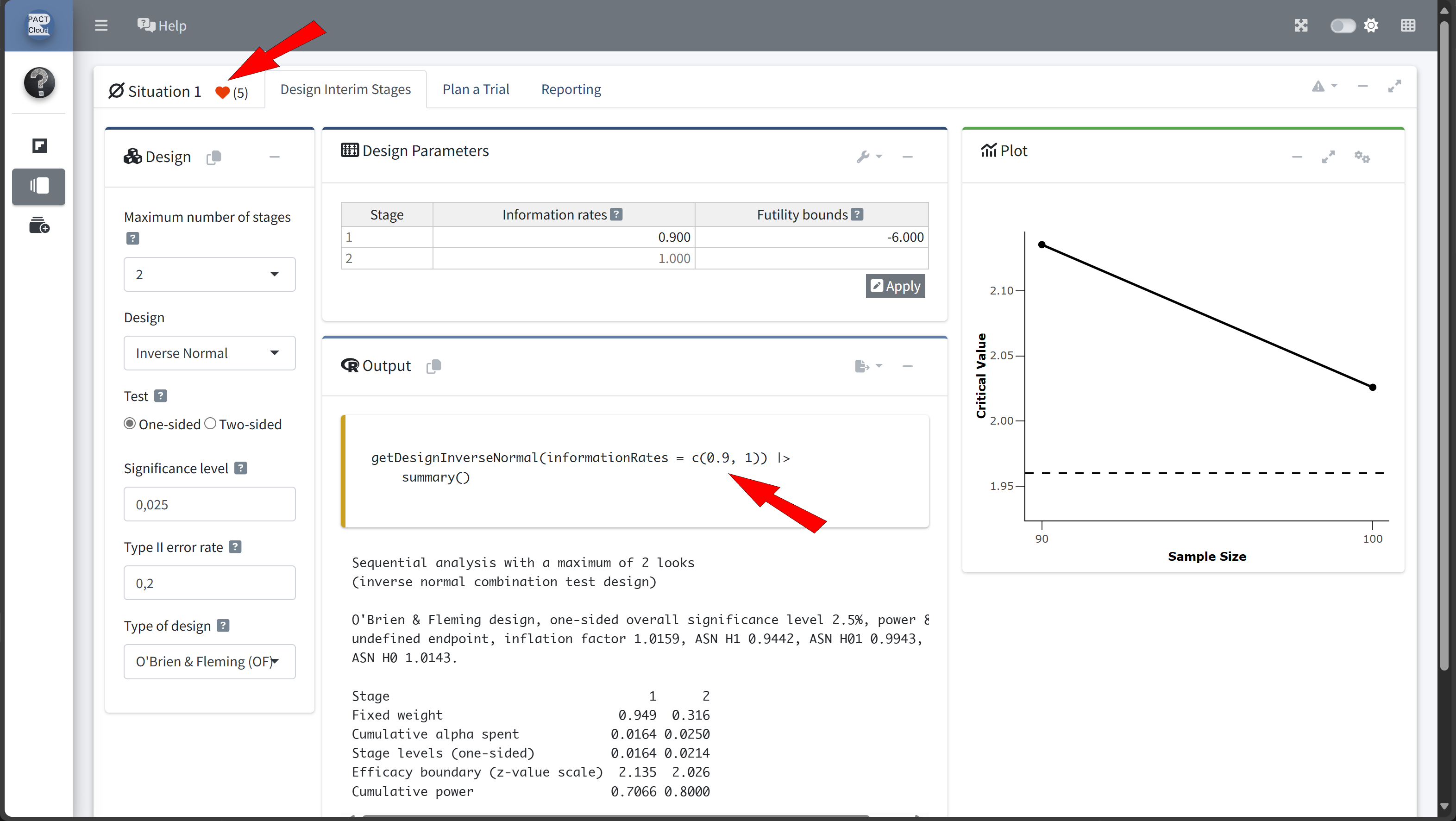
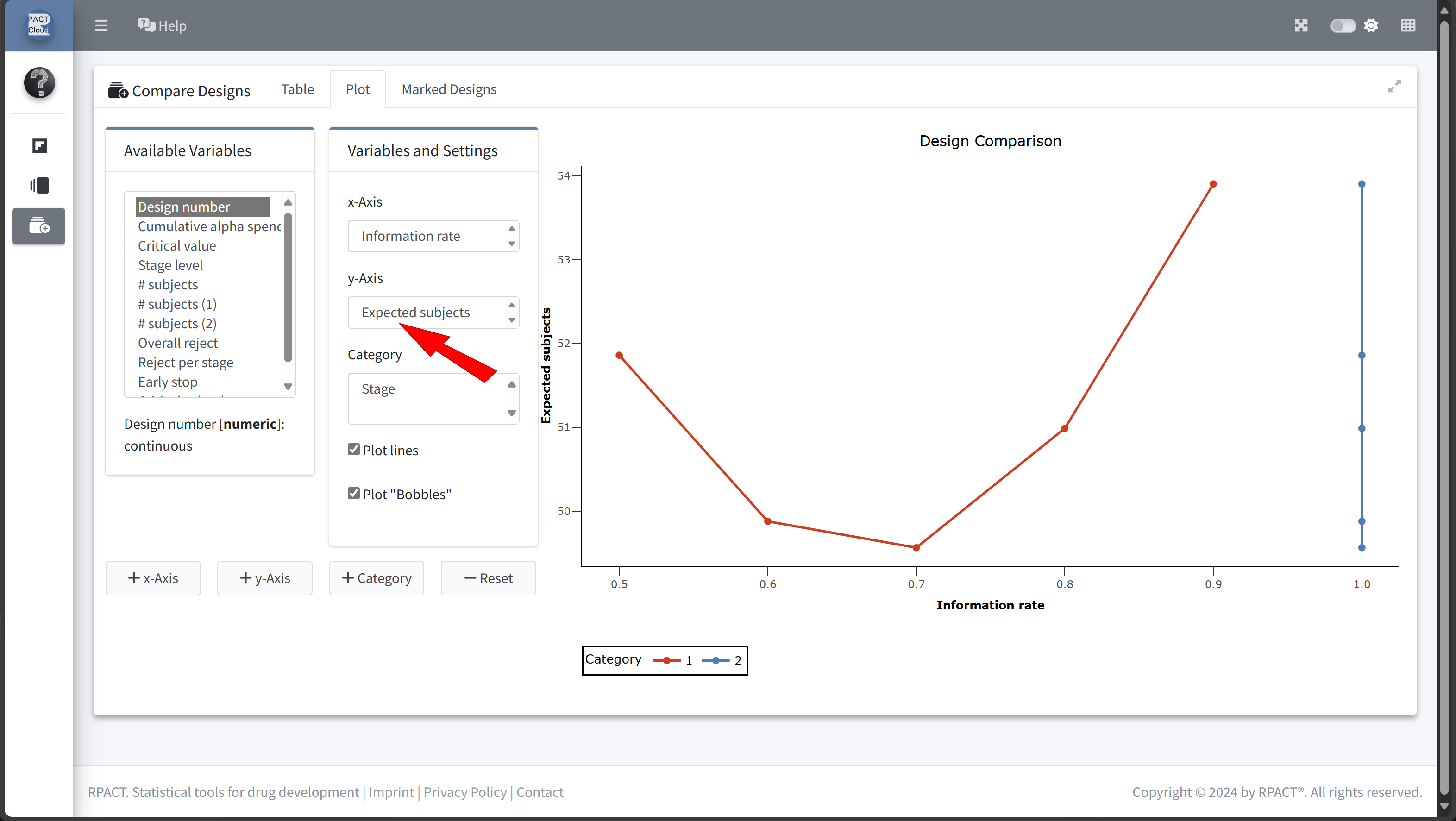
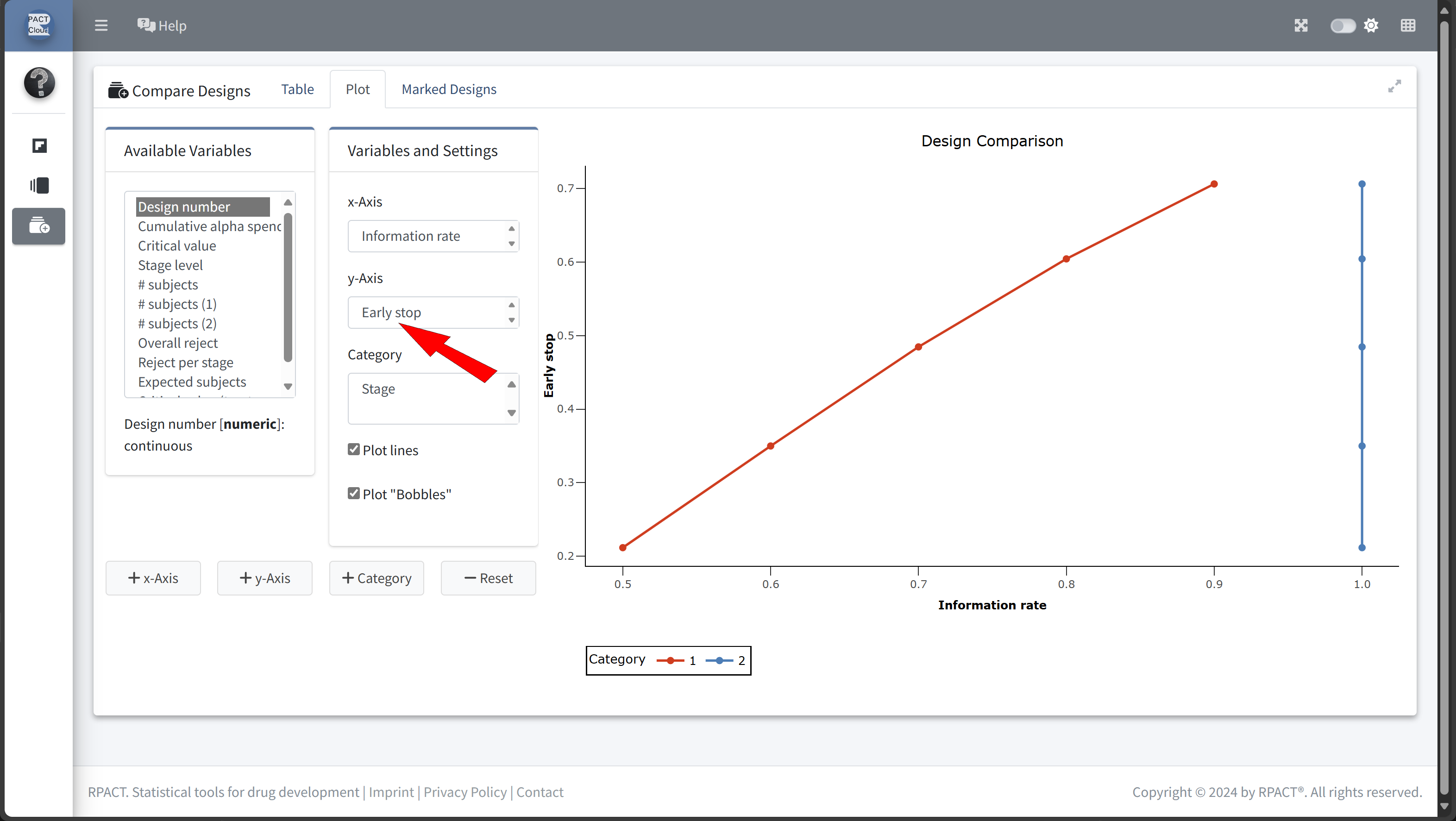
Design Comparison with RPACT Cloud
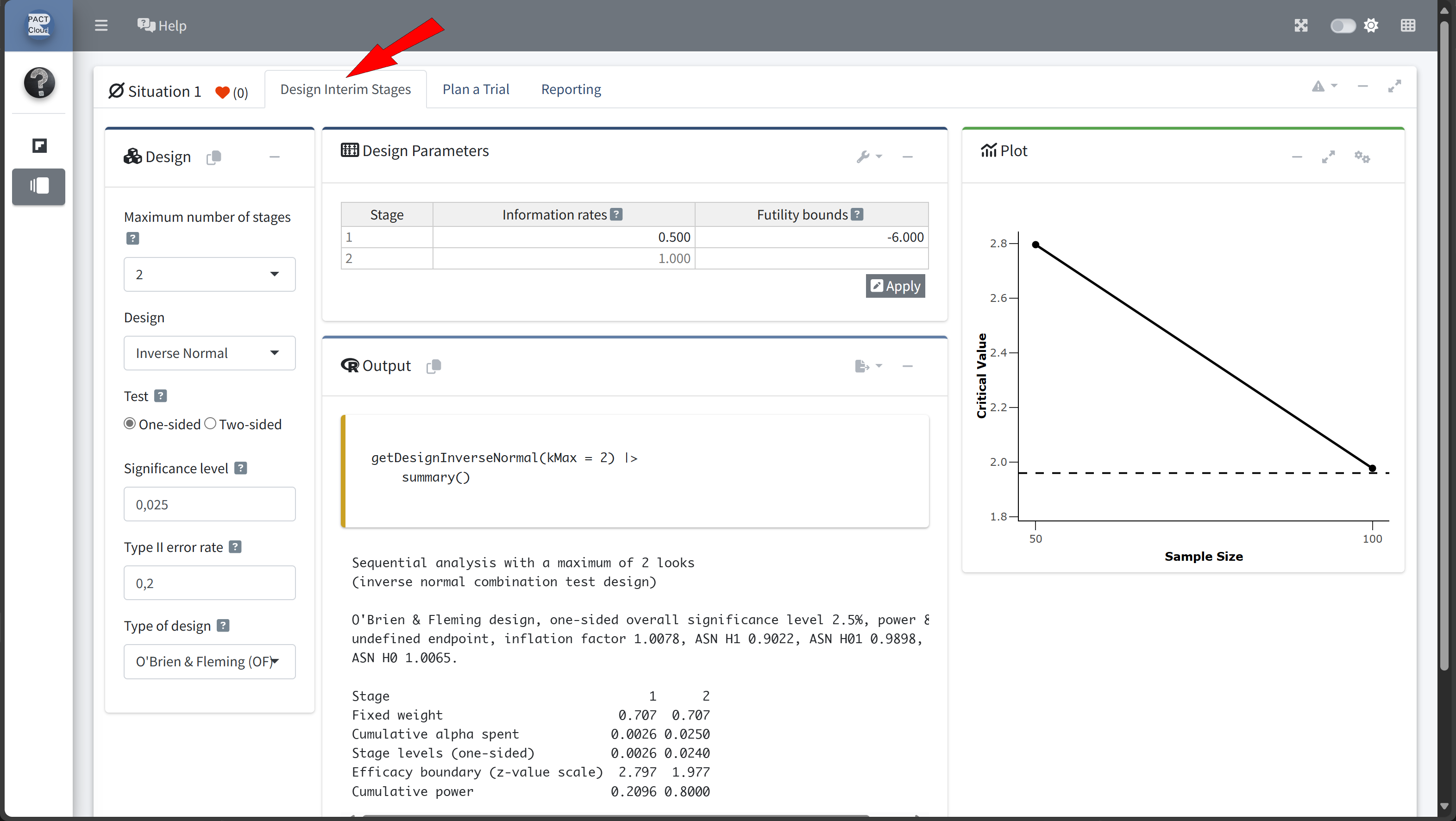
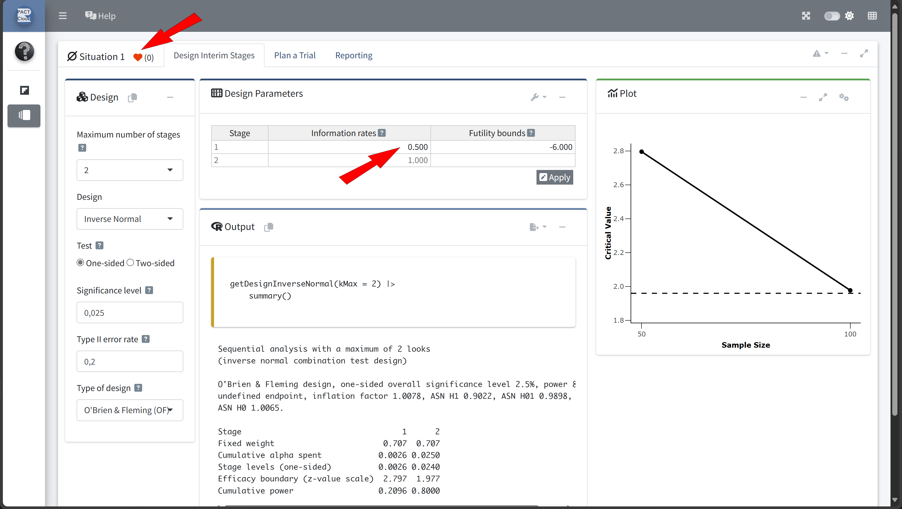

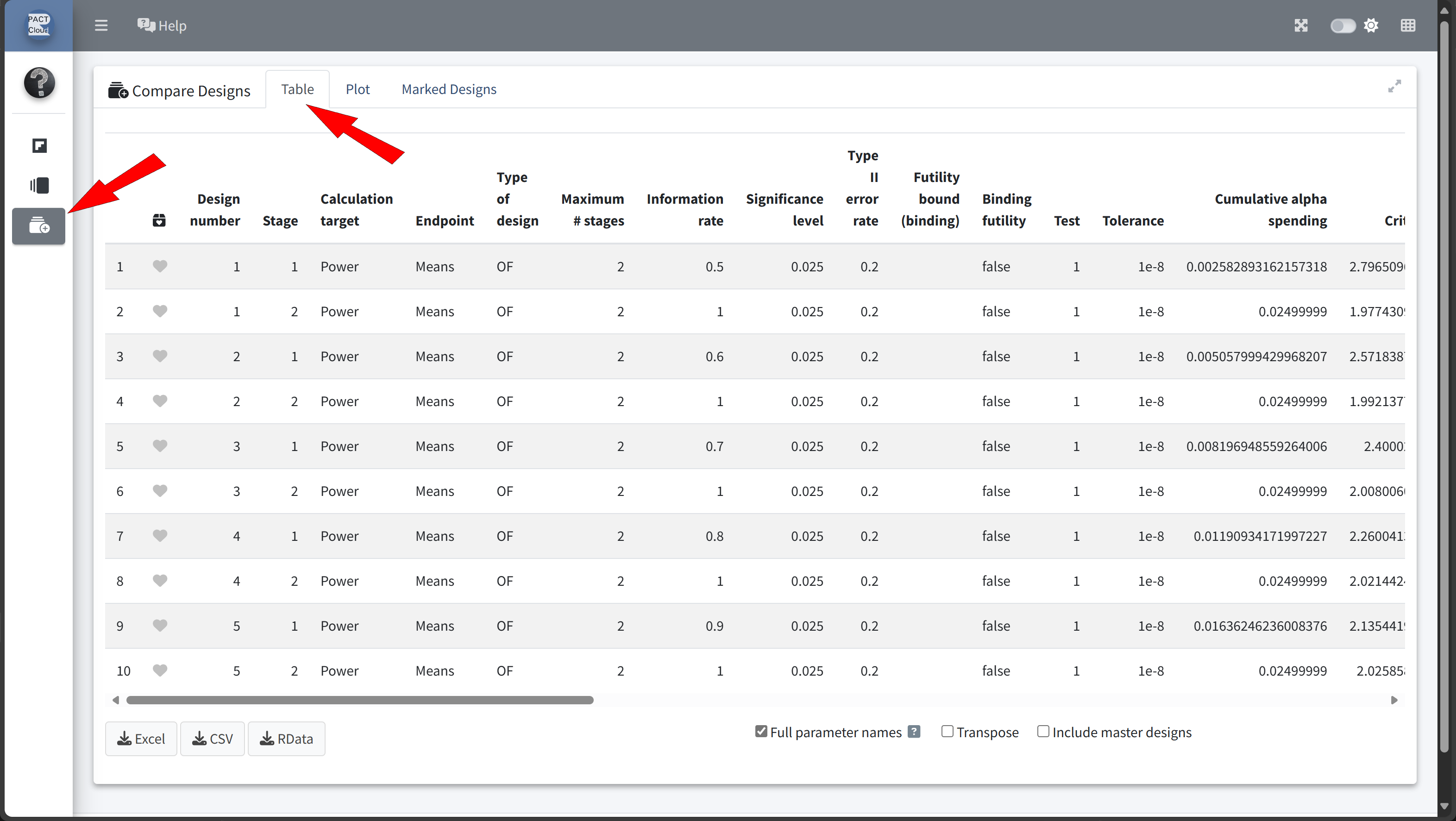
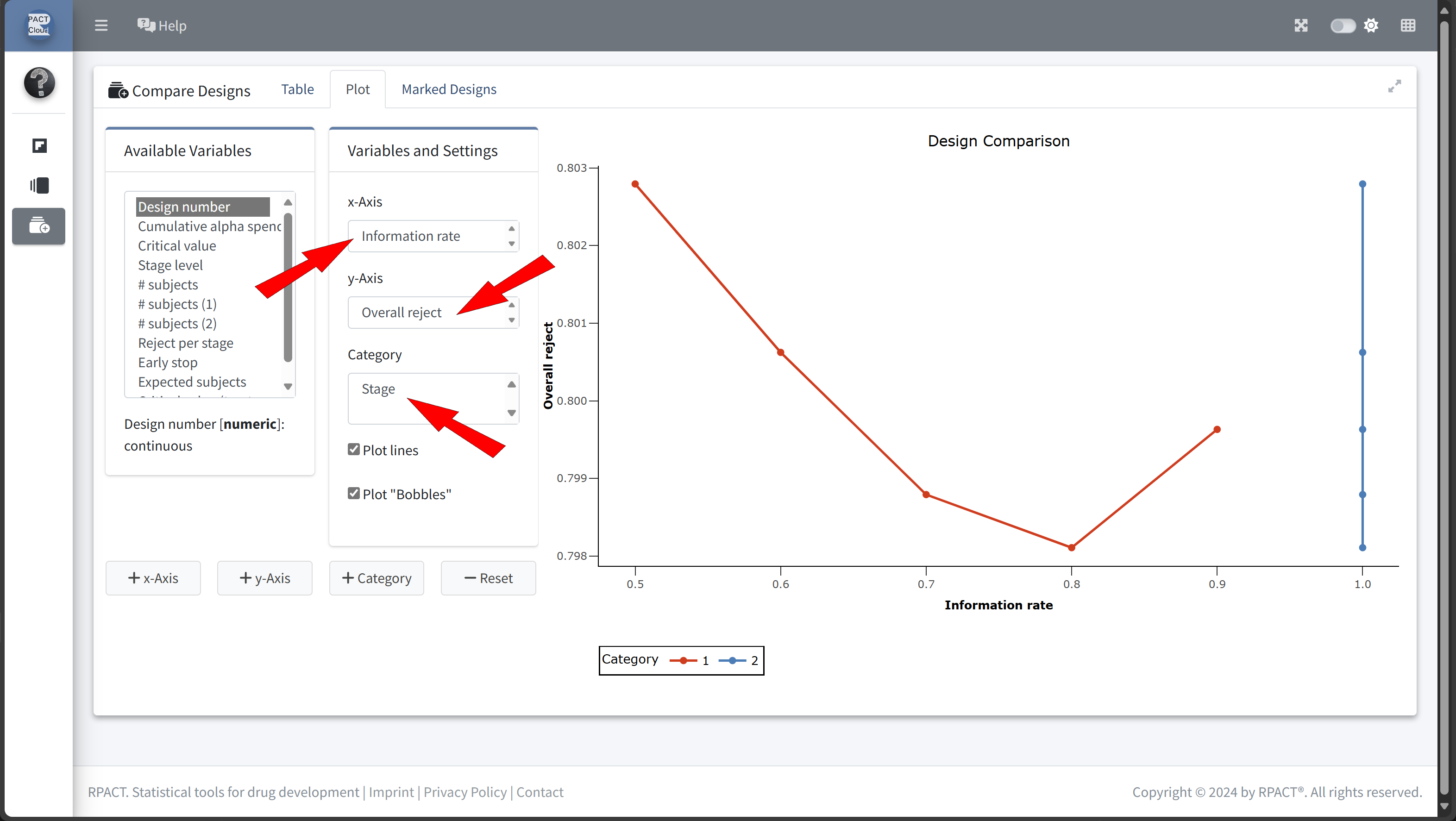
Here’s how to set up the design comparison in R:
# Run calculations for each scenario
results <- scenarios |>
lapply(function(scenario) {
getDesignGroupSequential(
informationRates = c(scenario$informationRate, 1),
alpha = 0.025,
sided = 1,
typeOfDesign = "OF"
) |>
getPowerMeans(
groups = 2,
alternative = 12,
stDev = 15,
maxNumberOfSubjects = numberOfSubjectsFixed, # 58
allocationRatioPlanned = 2
)
}
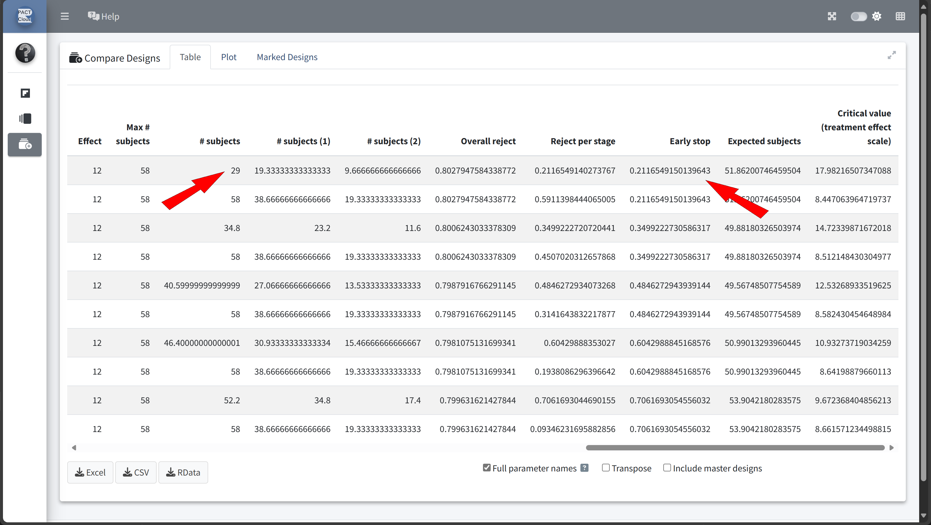
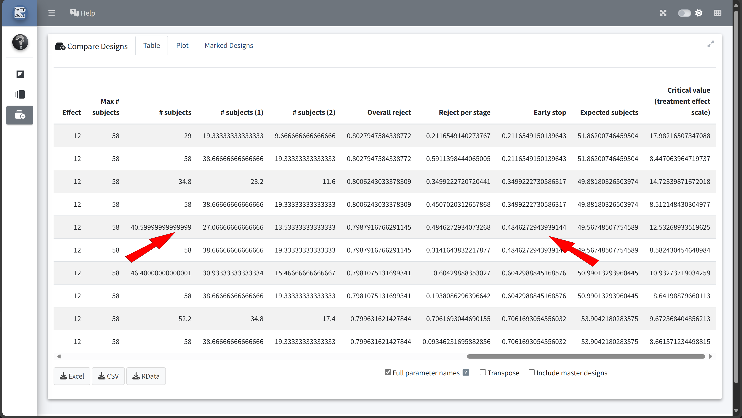
)| informationRate | expectedNumberOfSubjects | earlyStop | |
|---|---|---|---|
| Szenario 1 | 0.5 | 51.86201 | 0.2116549 |
| Szenario 2 | 0.6 | 49.88180 | 0.3499223 |
| Szenario 3 | 0.7 | 49.56749 | 0.4846273 |
| Szenario 4 | 0.8 | 50.99013 | 0.6042989 |
| Szenario 5 | 0.9 | 53.90422 | 0.7061693 |
In this example we decide to use information rate 0.7 because the expected number of subjects is lowest and the probability for an early stopping is nearly 50%.
Sample Size with an Interim Analysis
design <- getDesignGroupSequential(
informationRates = c(0.7, 1),
alpha = 0.025, # Overall significance level
beta = 0.2, # Power 80%
sided = 1, # One-sided test
typeOfDesign = "OF" # O'Brien & Fleming design
)
sampleSizeResult <- getSampleSizeMeans(
design = design,
groups = 2,
alternative = 12, # Expected difference
# (mean difference: 150 - 138 mmHg)
stDev = 15, # Common standard deviation
allocationRatioPlanned = 2 # 2:1 allocation
)
# Print the summary of the results
sampleSizeResult |> summary()
Sample size calculation for a continuous endpoint
Sequential analysis with a maximum of 2 looks (group sequential design), one-sided overall significance level 2.5%, power 80%. The results were calculated for a two-sample t-test, H0: mu(1) - mu(2) = 0, H1: effect = 12, standard deviation = 15, planned allocation ratio = 2.
| Stage | 1 | 2 |
|---|---|---|
| Planned information rate | 70% | 100% |
| Cumulative alpha spent | 0.0082 | 0.0250 |
| Stage levels (one-sided) | 0.0082 | 0.0223 |
| Efficacy boundary (z-value scale) | 2.400 | 2.008 |
| Efficacy boundary (t) | 12.508 | 8.566 |
| Cumulative power | 0.4861 | 0.8000 |
| Number of subjects | 40.7 | 58.2 |
| Expected number of subjects under H1 | 49.7 | |
| Exit probability for efficacy (under H0) | 0.0082 | |
| Exit probability for efficacy (under H1) | 0.4861 |
Legend:
- (t): treatment effect scale
Step 3: Calculate the Power of the Group-Sequential Design
To confirm that the design meets the target power while allowing for early stopping, we calculate the power of the study under the adjusted parameters:
powerResult <- getPowerMeans(
    design = design,
    groups = 2,
    alternative = 12,               # Expected effect size
    stDev = 15,                     # Common standard deviation
    # Sample size per stage from previous calculation
    maxNumberOfSubjects =
        ceiling(sampleSizeResult$numberOfSubjects)[2, 1],
    allocationRatioPlanned = 2     # Allocation ratio 2:1
)

# Print the summary of the results
powerResult |>
    summary()
Power calculation for a continuous endpoint
Sequential analysis with a maximum of 2 looks (group sequential design), one-sided overall significance level 2.5%. The results were calculated for a two-sample t-test, H0: mu(1) - mu(2) = 0, power directed towards larger values, H1: effect = 12, standard deviation = 15, maximum number of subjects = 59, planned allocation ratio = 2.
| Stage | 1 | 2 |
|---|---|---|
| Planned information rate | 70% | 100% |
| Cumulative alpha spent | 0.0082 | 0.0250 |
| Stage levels (one-sided) | 0.0082 | 0.0223 |
| Efficacy boundary (z-value scale) | 2.400 | 2.008 |
| Efficacy boundary (t) | 12.416 | 8.506 |
| Cumulative power | 0.4930 | 0.8057 |
| Number of subjects | 41.3 | 59.0 |
| Expected number of subjects under H1 | 50.3 | |
| Exit probability for efficacy (under H0) | 0.0082 | |
| Exit probability for efficacy (under H1) | 0.4930 |
Legend:
- (t): treatment effect scale
- Now we want to find a futility bound for the interim analysis that depends on a clinical relevant threshold.
- We assume that it makes no sense to continue the analysis when the treatment reduces the systolic blood pressure by 5 mmHg or less
- The minimum futility bound must be 0 because otherwise the effect would go in the wrong direction
- Ultimately, we want to use a boundary of 2 mmHg on treatment effect scale
# Run calculations for each scenario
results <- scenarios |>
    lapply(function(scenario) {
            getDesignGroupSequential(
                informationRates = c(0.7, 1),
                futilityBounds = scenario$futilityBounds,
                alpha = 0.025,
                sided = 1,
                typeOfDesign = "OF"
            ) |>
            getSampleSizeMeans(
                groups = 2,
                alternative = 12,
                stDev = 15,
                allocationRatioPlanned = 2
            )
    }
)
# Display results for each scenario
x <- sapply(results, function(result) {
result |> fetch("Futility bounds (treatment effect scale)")
})
#| echo: true
scenarios |>
bind_rows() |>
mutate("Futility bounds (treatment effect scale)" = x) |>
as.data.frame() |>
set_rownames(paste("Szenario", 1:length(x))) |>
kable()| futilityBounds | Futility bounds (treatment effect scale) | |
|---|---|---|
| Szenario 1 | -1.0 | -5.050045 |
| Szenario 2 | -0.5 | -2.512664 |
| Szenario 3 | 0.0 | 0 |
| Szenario 4 | 0.5 | 2.508815 |
| Szenario 5 | 1.0 | 4.97699 |
| Szenario 6 | 1.5 | 7.102175 |
Find Futility Bound Using stats::uniroot
One Dimensional Root (Zero) Finding
Description
The function uniroot searches the interval from lower to upper for a root (i.e., zero) of the function f with respect to its first argument.
soughtBoundaryTreatmentEffectScale <- 2
futilityBound <- uniroot(
    function(x) {
        soughtBoundaryTreatmentEffectScale -
            getDesignGroupSequential(
                informationRates = c(0.7, 1),
                futilityBounds = x,
                alpha = 0.025,
                sided = 1,
                typeOfDesign = "OF"
            ) |>
            getSampleSizeMeans(
                groups = 2,
                alternative = 12,
                stDev = 15,
                allocationRatioPlanned = 2
            ) |>
            fetch("Futility bounds (treatment effect scale)") |>
            as.numeric()
    },
    lower = 0,
    upper = 2
)$root
futilityBound
[1] 0.3985836Sample size calculation for a continuous endpoint
Sequential analysis with a maximum of 2 looks (group sequential design), one-sided overall significance level 2.5%, power 80%. The results were calculated for a two-sample t-test, H0: mu(1) - mu(2) = 0, H1: effect = 12, standard deviation = 15, planned allocation ratio = 2.
| Stage | 1 | 2 |
|---|---|---|
| Planned information rate | 70% | 100% |
| Cumulative alpha spent | 0.0082 | 0.0250 |
| Stage levels (one-sided) | 0.0082 | 0.0223 |
| Efficacy boundary (z-value scale) | 2.400 | 2.008 |
| Futility boundary (z-value scale) | 0.399 | |
| Efficacy boundary (t) | 12.496 | 8.558 |
| Futility boundary (t) | 2.000 | |
| Cumulative power | 0.4869 | 0.8000 |
| Number of subjects | 40.8 | 58.3 |
| Expected number of subjects under H1 | 49.4 | |
| Overall exit probability (under H0) | 0.6631 | |
| Overall exit probability (under H1) | 0.5114 | |
| Exit probability for efficacy (under H0) | 0.0082 | |
| Exit probability for efficacy (under H1) | 0.4869 | |
| Exit probability for futility (under H0) | 0.6549 | |
| Exit probability for futility (under H1) | 0.0245 |
Legend:
- (t): treatment effect scale
Thank you!
Questions and Answers