RPACT Multi-Arm Designs
November 13, 2025
RPACT Multi-Arm Designs

Theoretical Background of Adaptive Designs
Clue of Combination Testing Principle
Proposed by Peter Bauer (1989): Multistage testing with adaptive designs, in Biometrie und Informatik in Medizin und Biologie, Bauer and Köhne (1994) was the breakthrough.
Do not pool the data of the stages, combine the stage-wise \(p\,\)-values.
Then the distribution of the combination function under the null does not depend on design modifications, and the adaptive test is still a test at the level \(\alpha\) for the modified design.
In the two stages, even different hypotheses \(H_{01}\) and \(H_{02}\) can be considered, the considered global test is a test for \(H_0 = H_{01} \cap H_{02}\).
Or there are multiple hypotheses at the beginning of the trials and maybe some selected at interim.
Or there will be even hypotheses to be added at an interim stage (not of practical concern).
Clue of Combination Testing Principle
The rules for adapting the design need not be prespecified!
The combination test needs to be prespecified:
Bauer and Köhne (1994) proposed Fisher’s combination test (\(p_1 \cdot p_2\)) but also mentioned other combination tests, e.g., the inverse normal combination test (\(w_1 \Phi^{-1}(1 - p_1) + w_2 \Phi^{-1}(1 - p_2)\) ).
It was shown that the inverse normal combination test has the decisive advantage that then the adaptive confirmatory design simply generalizes the group sequential design (Lehmacher and Wassmer 1999).
So (initial) planning of an adaptive design is essentially the same as planning of a classical group sequential design and the same software can be used.
An equivalent procedure (not based on p-values but based on weighted \(Z\) score statistic) was proposed by Cui, Hung, and Wang (1999) .
Possible Data Dependent Changes of Design
Examples of data dependent changes of design are
Sample size recalculation
Change of allocation ratio
Change of test statistic
Flexible number of looks
Treatment arm selection (seamless phase II/III)
Population selection (population enrichment)
Selection of endpoints
For the latter three, in general, multiple hypotheses testing applies and a closed testing procedure can be used in order to control the experimentwise error rate in a strong sense.
Methods for Multi-Arm Multi-Stage (MAMS) Designs
Methods for predefined selection rules
(Stallard and Todd (2003), Magirr, Stallard, and Jaki (2014), …)
Flexible Multi-Stage Closed Combination Tests
(Bauer and Kieser (1999), Hommel (2001), …)
Do not require a predefined treatment and sample size selection rule.
Combine two methodology concepts:
Combination Tests and Closed Testing Principle.
Closed Testing Principle, 3 Hypotheses, select one
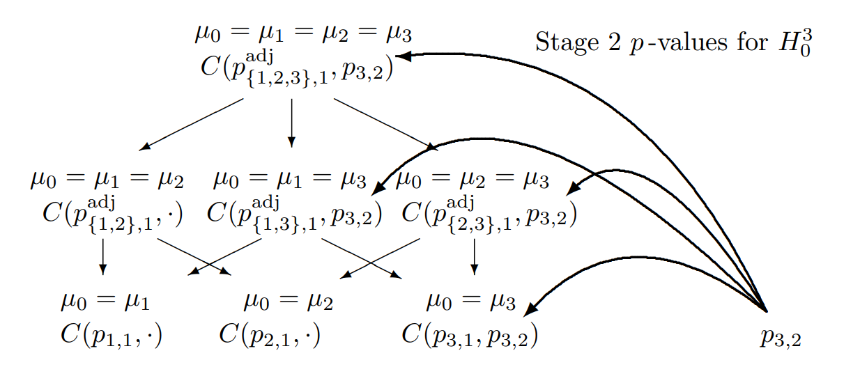
Combination tests to be performed for the closed system of hypotheses (\(G = 3\)) for testing hypothesis \(H_0^3\) if treatment arm 3 is selected for the second stage
Closed Testing Principle, 3 Hypotheses, select two
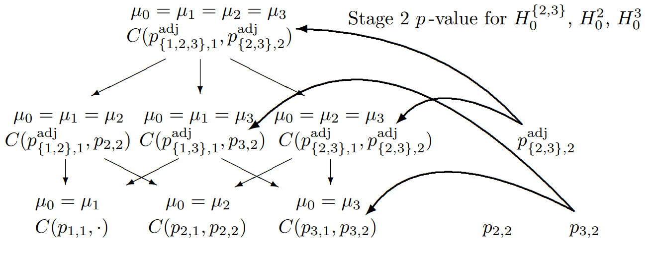
Combination tests to be performed for the closed system of hypotheses (\(G = 3\)) for testing hypothesis \(H_0^3\) if treatment arms 2 and 3 are selected for the second stage
Adaptive Designs with Treatment Arm Selection
Can be applied to selection of one or more than one treatment arm. The number of selected arms and the way of how to select treatment arms needs not to be preplanned.
Choice of combination test is free.
Data-driven recalculation of sample size is possible.
Choice of intersection tests is free. You can choose between Dunnett, Bonferroni, Simes, Sidak, hierarchical testing, etc.
For two-stage designs, the CRP principle can be applied: adaptive Dunnett test (König et al. (2008), Wassmer and Brannath (2016), Section 11.1.5, Mehta and Kappler (2025)).
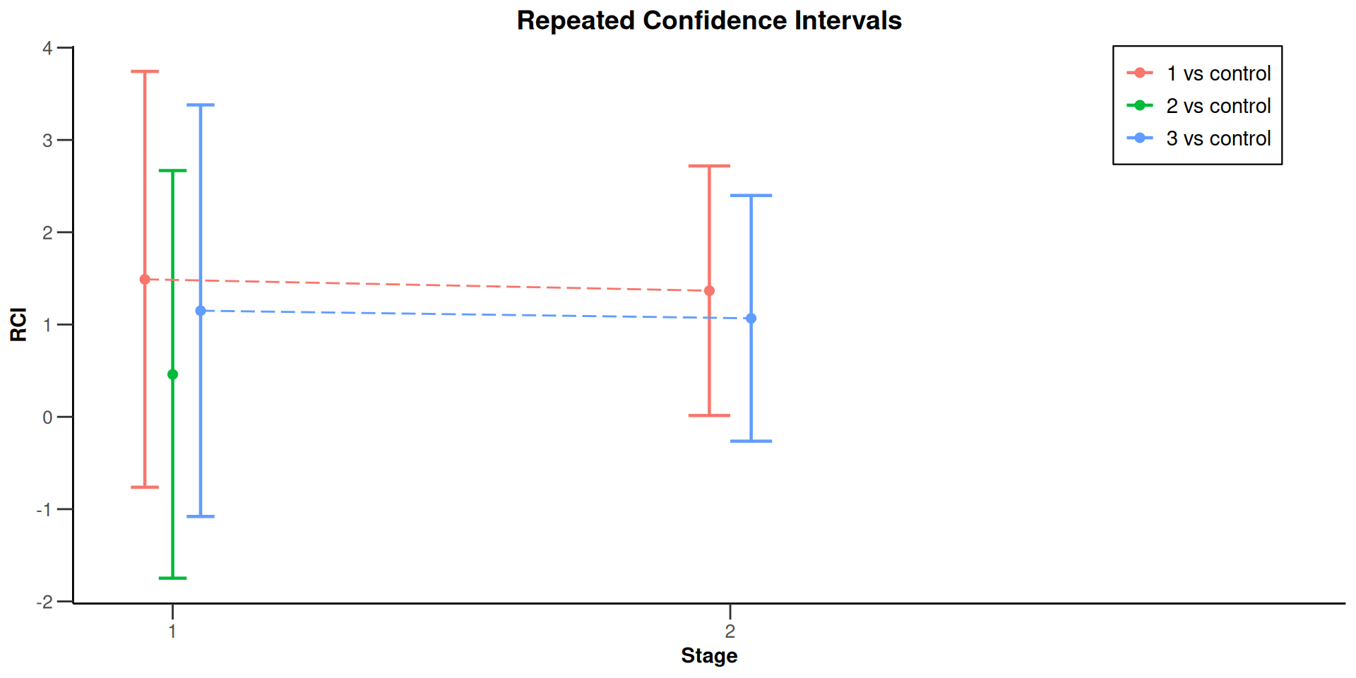
Confidence intervals based on stepwise testing are difficult to construct. This is a specific feature of multiple testing procedures and not of adaptive testing. Posch et al. (2005) proposed to construct repeated confidence intervals based on the single step adjusted overall p-values.
rpact Multi-Arm Analysis
Current Methods
Consider many-to-one comparisons comparing G active treatment arms to control.
Given a design and a dataset, at given stage the function
getAnalysisResults(design, dataInput, ...)calculates the results of the closed test procedure, overall p-values and test statistics, conditional rejection probability (CRP), conditional power, repeated confidence intervals (RCIs), and repeated overall p-values.
designis either fromgetDesignInverseNormal()orgetDesignFisher()(orNULL)For two stages,
design <- getDesignConditionalDunnett()can be selected.
Multi-Arm Analysis
The conditional power is calculated only if (at least) the sample size
nPlannedfor the subsequent stage(s) is specified.dataInputis the summary data used for calculating the test results. This is either an element ofDataSetMeans, ofDataSetRates, or ofDataSetSurvival.dataInputis defined throughgetDataset(), rpact identifies the type of endpoint.In rpact 3.0,
getDataset()is generalized to an arbitrary number of treatment arms.
Multi-Arm Analysis
dataInput
An element of
DataSetMeansfor one sample is created bygetDataset(means =, stDevs =, sampleSizes =)where
means, stDevs, sampleSizesare vectors with stagewise means, standard deviations, and sample sizes of length given by the number of available stages.An element of
DataSetMeansfor two samples is created bygetDataset(means1 =, means2 =, stDevs1 =, stDevs2 =, sampleSizes1 =, sampleSizes2 =)where
means1, means2, stDevs1, stDevs2, sampleSizes1, sampleSizes2are vectors with stagewise means, standard deviations, and sample sizes for the two treatment groups of length given by the number of available stages.
Multi-Arm Analysis
dataInput
An element of
DataSetMeansfor G + 1 samples is created bygetDataset(means1 =,..., means[G+1] =, stDevs1 =, ...,stDevs[G+1] =, sampleSizes1 =, ..., sampleSizes[G+1] =),where
means1, ..., means[G+1], stDevs1, ..., stDevs[G+1], sampleSizes1, ..., sampleSizes[G+1]are vectors with stagewise means, standard deviations, and sample sizes for G+1 treatment groups of length given by the number of available stages.Last treatment arm G + 1 always refers to the control group that cannot be deselected.
Only for the first stage all treatment arms needs to be specified, so treatment arm selection with an arbitrary number of treatment arms for subsequent stage can be considered.
Analogue definition of
DataSetRatesandDataSetSurvival.
Multi-Arm Analysis Example
Multi-Arm Analysis Example
Multi-Arm Analysis Example
Multi-arm analysis results (means of 4 groups, inverse normal combination test design)
Design parameters
- Fixed weights: 0.500, 0.500, 0.707
- Critical values: 2.904, 2.442, 2.053
- Futility bounds (non-binding): -Inf, -Inf
- Cumulative alpha spending: 0.001843, 0.008414, 0.025000
- Local one-sided significance levels: 0.001843, 0.007307, 0.020021
- Significance level: 0.0250
- Test: one-sided
Default parameters
- Normal approximation: FALSE
- Direction upper: TRUE
- Theta H0: 0
- Intersection test: Dunnett
- Variance option: overallPooled
Stage results
- Cumulative effect sizes (1): 1.490, 1.360, NA
- Cumulative effect sizes (2): 0.460, NA, NA
- Cumulative effect sizes (3): 1.150, 1.061, NA
- Cumulative (pooled) standard deviations (1): 2.197, 2.182, NA
- Cumulative (pooled) standard deviations (2): 2.134, NA, NA
- Cumulative (pooled) standard deviations (3): 2.373, 2.291, NA
- Stage-wise test statistics (1): 2.196, 2.038, NA
- Stage-wise test statistics (2): 0.691, NA, NA
- Stage-wise test statistics (3): 1.712, 1.647, NA
- Separate p-values (1): 0.01535, 0.02246, NA
- Separate p-values (2): 0.24552, NA, NA
- Separate p-values (3): 0.04516, 0.05176, NA
Adjusted stage-wise p-values
- Treatments 1, 2, 3 vs. control: 0.03904, 0.04112, NA
- Treatments 1, 2 vs. control: 0.02806, 0.02246, NA
- Treatments 1, 3 vs. control: 0.02810, 0.04112, NA
- Treatments 2, 3 vs. control: 0.07879, 0.05176, NA
- Treatment 1 vs. control: 0.01535, 0.02246, NA
- Treatment 2 vs. control: 0.24552, NA, NA
- Treatment 3 vs. control: 0.04516, 0.05176, NA
Overall adjusted test statistics
- Treatments 1, 2, 3 vs. control: 1.762, 2.475, NA
- Treatments 1, 2 vs. control: 1.910, 2.769, NA
- Treatments 1, 3 vs. control: 1.909, 2.579, NA
- Treatments 2, 3 vs. control: 1.413, 2.151, NA
- Treatment 1 vs. control: 2.161, 2.946, NA
- Treatment 2 vs. control: 0.689, NA, NA
- Treatment 3 vs. control: 1.694, 2.349, NA
Test actions
- Rejected (1): FALSE, TRUE, NA
- Rejected (2): FALSE, FALSE, NA
- Rejected (3): FALSE, FALSE, NA
Further analysis results
- Conditional rejection probability (1): 0.11367, 0.33392, NA
- Conditional rejection probability (2): 0.02593, NA, NA
- Conditional rejection probability (3): 0.07194, 0.22563, NA
- Conditional power (1): NA, NA, NA
- Conditional power (2): NA, NA, NA
- Conditional power (3): NA, NA, NA
- Repeated confidence intervals (lower) (1): -0.76273, 0.01443, NA
- Repeated confidence intervals (lower) (2): -1.74824, NA, NA
- Repeated confidence intervals (lower) (3): -1.07967, -0.26374, NA
- Repeated confidence intervals (upper) (1): 3.743, 2.719, NA
- Repeated confidence intervals (upper) (2): 2.668, NA, NA
- Repeated confidence intervals (upper) (3): 3.380, 2.399, NA
- Repeated p-values (1): 0.15176, 0.02326, NA
- Repeated p-values (2): 0.46577, NA, NA
- Repeated p-values (3): 0.23285, 0.04597, NA
Legend
- (i): results of treatment arm i vs. control group 4
Multi-Arm Analysis Example
Multi-Arm Analysis Example
Multi-arm analysis results for a continuous endpoint (3 active arms vs. control)
Sequential analysis with 3 looks (inverse normal combination test design), one-sided overall significance level 2.5%. The results were calculated using a multi-arm t-test, Dunnett intersection test, overall pooled variances option. H0: mu(i) - mu(control) = 0 against H1: mu(i) - mu(control) > 0.
| Stage | 1 | 2 | 3 |
|---|---|---|---|
| Fixed weight | 0.5 | 0.5 | 0.707 |
| Cumulative alpha spent | 0.0018 | 0.0084 | 0.0250 |
| Stage levels (one-sided) | 0.0018 | 0.0073 | 0.0200 |
| Efficacy boundary (z-value scale) | 2.904 | 2.442 | 2.053 |
| Cumulative effect size (1) | 1.490 | 1.360 | |
| Cumulative effect size (2) | 0.460 | ||
| Cumulative effect size (3) | 1.150 | 1.061 | |
| Cumulative (pooled) standard deviation | 2.276 | 2.263 | |
| Stage-wise test statistic (1) | 2.196 | 2.038 | |
| Stage-wise test statistic (2) | 0.691 | ||
| Stage-wise test statistic (3) | 1.712 | 1.647 | |
| Stage-wise p-value (1) | 0.0153 | 0.0225 | |
| Stage-wise p-value (2) | 0.2455 | ||
| Stage-wise p-value (3) | 0.0452 | 0.0518 | |
| Adjusted stage-wise p-value (1, 2, 3) | 0.0390 | 0.0411 | |
| Adjusted stage-wise p-value (1, 2) | 0.0281 | 0.0225 | |
| Adjusted stage-wise p-value (1, 3) | 0.0281 | 0.0411 | |
| Adjusted stage-wise p-value (2, 3) | 0.0788 | 0.0518 | |
| Adjusted stage-wise p-value (1) | 0.0153 | 0.0225 | |
| Adjusted stage-wise p-value (2) | 0.2455 | ||
| Adjusted stage-wise p-value (3) | 0.0452 | 0.0518 | |
| Overall adjusted test statistic (1, 2, 3) | 1.762 | 2.475 | |
| Overall adjusted test statistic (1, 2) | 1.910 | 2.769 | |
| Overall adjusted test statistic (1, 3) | 1.909 | 2.579 | |
| Overall adjusted test statistic (2, 3) | 1.413 | 2.151 | |
| Overall adjusted test statistic (1) | 2.161 | 2.946 | |
| Overall adjusted test statistic (2) | 0.689 | ||
| Overall adjusted test statistic (3) | 1.694 | 2.349 | |
| Test action: reject (1) | FALSE | TRUE | |
| Test action: reject (2) | FALSE | FALSE | |
| Test action: reject (3) | FALSE | FALSE | |
| Conditional rejection probability (1) | 0.1137 | 0.3339 | |
| Conditional rejection probability (2) | 0.0259 | ||
| Conditional rejection probability (3) | 0.0719 | 0.2256 | |
| 95% repeated confidence interval (1) | [-0.763; 3.743] | [0.014; 2.719] | |
| 95% repeated confidence interval (2) | [-1.748; 2.668] | ||
| 95% repeated confidence interval (3) | [-1.080; 3.380] | [-0.264; 2.399] | |
| Repeated p-value (1) | 0.1518 | 0.0233 | |
| Repeated p-value (2) | 0.4658 | ||
| Repeated p-value (3) | 0.2329 | 0.0460 |
Legend:
- (i): results of treatment arm i vs. control arm
- (i, j, …): comparison of treatment arms ‘i, j, …’ vs. control arm
Multi-Arm Analysis Example
Multi-Arm Analysis Example
Conditional Power
Multi-Arm Analysis Example
Multi-arm analysis results for a continuous endpoint (3 active arms vs. control)
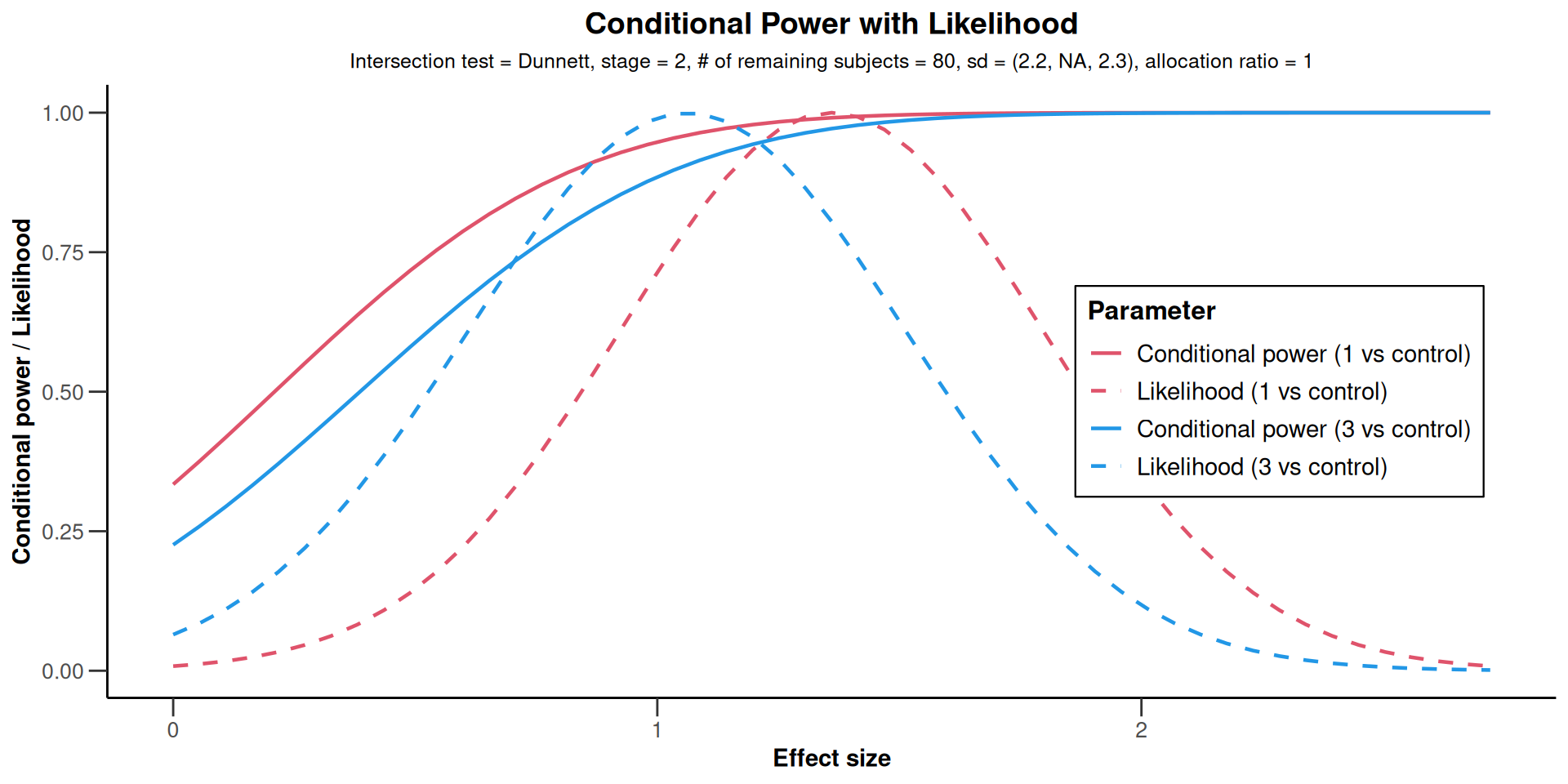
Sequential analysis with 3 looks (inverse normal combination test design), one-sided overall significance level 2.5%. The results were calculated using a multi-arm t-test, Dunnett intersection test, overall pooled variances option. H0: mu(i) - mu(control) = 0 against H1: mu(i) - mu(control) > 0. The conditional power calculation with planned sample size is based on overall effect: thetaH1(1) = 1.36, thetaH1(2) = NA, thetaH1(3) = 1.06 and overall standard deviation: sd(1) = 2.18, sd(2) = NA, sd(3) = 2.29.
| Stage | 1 | 2 | 3 |
|---|---|---|---|
| Fixed weight | 0.5 | 0.5 | 0.707 |
| Cumulative alpha spent | 0.0018 | 0.0084 | 0.0250 |
| Stage levels (one-sided) | 0.0018 | 0.0073 | 0.0200 |
| Efficacy boundary (z-value scale) | 2.904 | 2.442 | 2.053 |
| Cumulative effect size (1) | 1.490 | 1.360 | |
| Cumulative effect size (2) | 0.460 | ||
| Cumulative effect size (3) | 1.150 | 1.061 | |
| Cumulative (pooled) standard deviation | 2.276 | 2.263 | |
| Stage-wise test statistic (1) | 2.196 | 2.038 | |
| Stage-wise test statistic (2) | 0.691 | ||
| Stage-wise test statistic (3) | 1.712 | 1.647 | |
| Stage-wise p-value (1) | 0.0153 | 0.0225 | |
| Stage-wise p-value (2) | 0.2455 | ||
| Stage-wise p-value (3) | 0.0452 | 0.0518 | |
| Adjusted stage-wise p-value (1, 2, 3) | 0.0390 | 0.0411 | |
| Adjusted stage-wise p-value (1, 2) | 0.0281 | 0.0225 | |
| Adjusted stage-wise p-value (1, 3) | 0.0281 | 0.0411 | |
| Adjusted stage-wise p-value (2, 3) | 0.0788 | 0.0518 | |
| Adjusted stage-wise p-value (1) | 0.0153 | 0.0225 | |
| Adjusted stage-wise p-value (2) | 0.2455 | ||
| Adjusted stage-wise p-value (3) | 0.0452 | 0.0518 | |
| Overall adjusted test statistic (1, 2, 3) | 1.762 | 2.475 | |
| Overall adjusted test statistic (1, 2) | 1.910 | 2.769 | |
| Overall adjusted test statistic (1, 3) | 1.909 | 2.579 | |
| Overall adjusted test statistic (2, 3) | 1.413 | 2.151 | |
| Overall adjusted test statistic (1) | 2.161 | 2.946 | |
| Overall adjusted test statistic (2) | 0.689 | ||
| Overall adjusted test statistic (3) | 1.694 | 2.349 | |
| Test action: reject (1) | FALSE | TRUE | |
| Test action: reject (2) | FALSE | FALSE | |
| Test action: reject (3) | FALSE | FALSE | |
| Conditional rejection probability (1) | 0.1137 | 0.3339 | |
| Conditional rejection probability (2) | 0.0259 | ||
| Conditional rejection probability (3) | 0.0719 | 0.2256 | |
| Planned sample size | 80 | ||
| Conditional power (1) | 0.9908 | ||
| Conditional power (2) | |||
| Conditional power (3) | 0.9064 | ||
| 95% repeated confidence interval (1) | [-0.763; 3.743] | [0.014; 2.719] | |
| 95% repeated confidence interval (2) | [-1.748; 2.668] | ||
| 95% repeated confidence interval (3) | [-1.080; 3.380] | [-0.264; 2.399] | |
| Repeated p-value (1) | 0.1518 | 0.0233 | |
| Repeated p-value (2) | 0.4658 | ||
| Repeated p-value (3) | 0.2329 | 0.0460 |
Legend:
- (i): results of treatment arm i vs. control arm
- (i, j, …): comparison of treatment arms ‘i, j, …’ vs. control arm
Multi-Arm Analysis Example
Conditional Power
Multi-Arm Analysis Example
Final stage
exampleMeans <- getDataset(
    n1      = c( 23,  25, NA),
    n2      = c( 25,  NA, NA),
    n3      = c( 24,  27, 42),
    n4      = c( 22,  29, 47),
    means1  = c(2.41, 2.27, NA),
    means2  = c(1.38,  NA, NA),
    means3  = c(2.07, 2.01, 2.05),
    means4  = c(0.92, 1.02, 1.05),
    stDevs1 = c(2.24, 2.21, NA),
    stDevs2 = c(2.12,  NA, NA),
    stDevs3 = c(2.56, 2.32, 2.15),
    stDevs4 = c(2.15, 2.21, 2.09)
)

designIN |> getAnalysisResults(
  dataInput = exampleMeans
) |> summary()
Multi-Arm Analysis Example
Multi-arm analysis results for a continuous endpoint (3 active arms vs. control)
Sequential analysis with 3 looks (inverse normal combination test design), one-sided overall significance level 2.5%. The results were calculated using a multi-arm t-test, Dunnett intersection test, overall pooled variances option. H0: mu(i) - mu(control) = 0 against H1: mu(i) - mu(control) > 0.
| Stage | 1 | 2 | 3 |
|---|---|---|---|
| Fixed weight | 0.5 | 0.5 | 0.707 |
| Cumulative alpha spent | 0.0018 | 0.0084 | 0.0250 |
| Stage levels (one-sided) | 0.0018 | 0.0073 | 0.0200 |
| Efficacy boundary (z-value scale) | 2.904 | 2.442 | 2.053 |
| Cumulative effect size (1) | 1.490 | 1.360 | |
| Cumulative effect size (2) | 0.460 | ||
| Cumulative effect size (3) | 1.150 | 1.061 | 1.032 |
| Cumulative (pooled) standard deviation | 2.276 | 2.263 | 2.201 |
| Stage-wise test statistic (1) | 2.196 | 2.038 | |
| Stage-wise test statistic (2) | 0.691 | ||
| Stage-wise test statistic (3) | 1.712 | 1.647 | 2.223 |
| Stage-wise p-value (1) | 0.0153 | 0.0225 | |
| Stage-wise p-value (2) | 0.2455 | ||
| Stage-wise p-value (3) | 0.0452 | 0.0518 | 0.0144 |
| Adjusted stage-wise p-value (1, 2, 3) | 0.0390 | 0.0411 | 0.0144 |
| Adjusted stage-wise p-value (1, 2) | 0.0281 | 0.0225 | |
| Adjusted stage-wise p-value (1, 3) | 0.0281 | 0.0411 | 0.0144 |
| Adjusted stage-wise p-value (2, 3) | 0.0788 | 0.0518 | 0.0144 |
| Adjusted stage-wise p-value (1) | 0.0153 | 0.0225 | |
| Adjusted stage-wise p-value (2) | 0.2455 | ||
| Adjusted stage-wise p-value (3) | 0.0452 | 0.0518 | 0.0144 |
| Overall adjusted test statistic (1, 2, 3) | 1.762 | 2.475 | 3.296 |
| Overall adjusted test statistic (1, 2) | 1.910 | 2.769 | |
| Overall adjusted test statistic (1, 3) | 1.909 | 2.579 | 3.369 |
| Overall adjusted test statistic (2, 3) | 1.413 | 2.151 | 3.066 |
| Overall adjusted test statistic (1) | 2.161 | 2.946 | |
| Overall adjusted test statistic (2) | 0.689 | ||
| Overall adjusted test statistic (3) | 1.694 | 2.349 | 3.207 |
| Test action: reject (1) | FALSE | TRUE | TRUE |
| Test action: reject (2) | FALSE | FALSE | FALSE |
| Test action: reject (3) | FALSE | FALSE | TRUE |
| Conditional rejection probability (1) | 0.1137 | 0.3339 | |
| Conditional rejection probability (2) | 0.0259 | ||
| Conditional rejection probability (3) | 0.0719 | 0.2256 | |
| 95% repeated confidence interval (1) | [-0.763; 3.743] | [0.014; 2.719] | |
| 95% repeated confidence interval (2) | [-1.748; 2.668] | ||
| 95% repeated confidence interval (3) | [-1.080; 3.380] | [-0.264; 2.399] | [0.244; 1.827] |
| Repeated p-value (1) | 0.1518 | 0.0233 | |
| Repeated p-value (2) | 0.4658 | ||
| Repeated p-value (3) | 0.2329 | 0.0460 | 0.0012 |
Legend:
- (i): results of treatment arm i vs. control arm
- (i, j, …): comparison of treatment arms ‘i, j, …’ vs. control arm
rpact Multi-Arm Simulation
Overview
getSimulationMultiArmMeans(design,...),
getSimulationMultiArmRates(design,...), and
getSimulationMultiArmSurvival(design,...)
perform simulations in multi-arm designs for testing means, rates, and hazard ratios, respectively.
You can assess different treatment arm selection strategies, sample size reassessment methods, general stopping, and stopping for futility rules.
Define selection strategy and effect size pattern appropriately (e.g., linear, sigmoidEmax, user defined, etc).
Time to Event example:
Time to disease progression event
2 active arms, 1 control arm
Equal allocation between groups
Power 90%
\(\alpha\) = 0.025 one sided
2 analyses (1 IA at 50% events) futility analysis at interim and select best dose based on highest HR
Assume median TTE in control arm: 25 months
Median TTE in active: 18 months so target HR 0.72
Accrual: Assume 10 for first 10 months, then 20 for next 10 then 30 per month thereafter for max 36 months (or feel free to use a constant accrual rate)
Sample Size Calculation
Around 390 events are needed to achieve 90% power for a two-sample comparison:
Sample size calculation for a survival endpoint
Fixed sample analysis, one-sided significance level 2.5%, power 90%. The results were calculated for a two-sample logrank test, H0: hazard ratio = 1, H1: hazard ratio = 0.72, control median(2) = 25, accrual time = c(10, 20, 36), accrual intensity = c(10, 20, 30).
| Stage | Fixed |
|---|---|
| Stage level (one-sided) | 0.0250 |
| Efficacy boundary (z-value scale) | 1.960 |
| Efficacy boundary (t) | 0.820 |
| Number of subjects | 780.0 |
| Number of events | 389.5 |
| Analysis time | 52.02 |
| Expected study duration under H1 | 52.02 |
Legend:
- (t): treatment effect scale
Design with Interim Stage and Bonferroni
Design with Interim Stage and Bonferroni
Sample size calculation for a survival endpoint
Sequential analysis with a maximum of 2 looks (inverse normal combination test design), one-sided overall significance level 1.25%, power 90%. The results were calculated for a two-sample logrank test, H0: hazard ratio = 1, H1: hazard ratio = 0.72, control median(2) = 25, accrual time = c(10, 20, 36), accrual intensity = c(10, 20, 30).
| Stage | 1 | 2 |
|---|---|---|
| Fixed weight | 0.707 | 0.707 |
| Cumulative alpha spent | 0 | 0.0125 |
| Stage levels (one-sided) | 0 | 0.0125 |
| Efficacy boundary (z-value scale) | Inf | 2.241 |
| Futility boundary (z-value scale) | 0 | |
| Efficacy boundary (t) | 0 | 0.812 |
| Futility boundary (t) | 1.000 | |
| Cumulative power | 0 | 0.9000 |
| Number of subjects | 780.0 | 780.0 |
| Expected number of subjects under H1 | 780.0 | |
| Cumulative number of events | 230.8 | 461.6 |
| Expected number of events under H1 | 460.2 | |
| Analysis time | 37.53 | 60.77 |
| Expected study duration under H1 | 60.62 | |
| Overall exit probability (under H0) | 0.5000 | |
| Overall exit probability (under H1) | 0.0063 | |
| Exit probability for efficacy (under H0) | 0 | |
| Exit probability for efficacy (under H1) | 0 | |
| Exit probability for futility (under H0) | 0.5000 | |
| Exit probability for futility (under H1) | 0.0063 |
Legend:
- (t): treatment effect scale
A Multi-Arm Approach
Based on this result, we plan a multi-arm design with a maximum of 460 events in order to achieve power 90%
The procedure is designed in such a way that in case of selecting a treatment arm the specified events need to be observed for the remaining arms (i.e., no event number recalculation)
Note, for multi-armed designs, to simulate TTE on a patient level is not available yet. However, in rpact the approach of Deng et al. (2019) for simulating normally distributed log-rank statistics is implemented
The number of events for pairwise comparisons are estimated from the assumption about the hazard ratios
This provides a reasonable approximation for the assessment of test characteristics, i.e., for the estimation of power and selection probabilities.
Example Select All
design <- getDesignInverseNormal(
    kMax = 2,
    typeOfDesign = "noEarlyEfficacy",
    alpha = 0.025,
    futilityBounds = 0
)
effectMatrix = matrix(
    c(0.72, 0.72,
    0.72, 0.8,
    0.72, 0.9,
    0.8, 0.8,
    0.8, 0.9,
    1, 1),
    ncol = 2, byrow = TRUE
)
design |> getSimulationMultiArmSurvival(
    activeArms = 2,
    directionUpper = FALSE,
    typeOfShape = "userDefined",
    effectMatrix = effectMatrix,
    typeOfSelection = "all",
    plannedEvents = c(230, 460),
    maxNumberOfIterations = 1000,
    seed = 123
) |> summary()
Example Select All
Simulation of a survival endpoint (multi-arm design)
Sequential analysis with a maximum of 2 looks (inverse normal combination test design), one-sided overall significance level 2.5%. The results were simulated for a multi-arm logrank test (2 treatments vs. control), H0: hazard ratio(i) = 1, power directed towards smaller values, H1: omega_max as specified, planned cumulative events = c(230, 460), effect shape = user defined, intersection test = Dunnett, selection = all, effect measure based on effect estimate, success criterion: all, simulation runs = 1000, seed = 123.
| Stage | 1 | 2 |
|---|---|---|
| Fixed weight | 0.707 | 0.707 |
| Cumulative alpha spent | 0 | 0.0250 |
| Stage levels (one-sided) | 0 | 0.0250 |
| Efficacy boundary (z-value scale) | Inf | 1.960 |
| Futility boundary (z-value scale) | 0 | |
| Reject at least one [1] | 0.9080 | |
| Reject at least one [2] | 0.8020 | |
| Reject at least one [3] | 0.6990 | |
| Reject at least one [4] | 0.5770 | |
| Reject at least one [5] | 0.3670 | |
| Reject at least one [6] | 0.0190 | |
| Rejected arms per stage [1] | ||
| Treatment arm 1 vs. control | 0 | 0.8290 |
| Treatment arm 2 vs. control | 0 | 0.8240 |
| Rejected arms per stage [2] | ||
| Treatment arm 1 vs. control | 0 | 0.7630 |
| Treatment arm 2 vs. control | 0 | 0.4990 |
| Rejected arms per stage [3] | ||
| Treatment arm 1 vs. control | 0 | 0.6930 |
| Treatment arm 2 vs. control | 0 | 0.1530 |
| Rejected arms per stage [4] | ||
| Treatment arm 1 vs. control | 0 | 0.4490 |
| Treatment arm 2 vs. control | 0 | 0.4580 |
| Rejected arms per stage [5] | ||
| Treatment arm 1 vs. control | 0 | 0.3510 |
| Treatment arm 2 vs. control | 0 | 0.1170 |
| Rejected arms per stage [6] | ||
| Treatment arm 1 vs. control | 0 | 0.0150 |
| Treatment arm 2 vs. control | 0 | 0.0110 |
| Success per stage [1] | 0 | 0.7450 |
| Success per stage [2] | 0 | 0.4600 |
| Success per stage [3] | 0 | 0.1470 |
| Success per stage [4] | 0 | 0.3300 |
| Success per stage [5] | 0 | 0.1010 |
| Success per stage [6] | 0 | 0.0070 |
| Cumulative number of events [1] | ||
| Treatment arm 1 vs. control | 162.1 | 324.3 |
| Treatment arm 2 vs. control | 162.1 | 324.3 |
| Cumulative number of events [2] | ||
| Treatment arm 1 vs. control | 157.0 | 314.0 |
| Treatment arm 2 vs. control | 164.3 | 328.6 |
| Cumulative number of events [3] | ||
| Treatment arm 1 vs. control | 151.0 | 302.0 |
| Treatment arm 2 vs. control | 166.8 | 333.6 |
| Cumulative number of events [4] | ||
| Treatment arm 1 vs. control | 159.2 | 318.5 |
| Treatment arm 2 vs. control | 159.2 | 318.5 |
| Cumulative number of events [5] | ||
| Treatment arm 1 vs. control | 153.3 | 306.7 |
| Treatment arm 2 vs. control | 161.9 | 323.7 |
| Cumulative number of events [6] | ||
| Treatment arm 1 vs. control | 153.3 | 306.7 |
| Treatment arm 2 vs. control | 153.3 | 306.7 |
| Expected number of events under H1 [1] | 458.6 | |
| Expected number of events under H1 [2] | 456.1 | |
| Expected number of events under H1 [3] | 449.9 | |
| Expected number of events under H1 [4] | 445.5 | |
| Expected number of events under H1 [5] | 431.5 | |
| Expected number of events under H1 [6] | 345.7 | |
| Overall exit probability [1] | 0.0060 | |
| Overall exit probability [2] | 0.0170 | |
| Overall exit probability [3] | 0.0440 | |
| Overall exit probability [4] | 0.0630 | |
| Overall exit probability [5] | 0.1240 | |
| Overall exit probability [6] | 0.4970 | |
| Selected arms [1] | ||
| Treatment arm 1 vs. control | 1.0000 | 0.9940 |
| Treatment arm 2 vs. control | 1.0000 | 0.9940 |
| Selected arms [2] | ||
| Treatment arm 1 vs. control | 1.0000 | 0.9830 |
| Treatment arm 2 vs. control | 1.0000 | 0.9830 |
| Selected arms [3] | ||
| Treatment arm 1 vs. control | 1.0000 | 0.9560 |
| Treatment arm 2 vs. control | 1.0000 | 0.9560 |
| Selected arms [4] | ||
| Treatment arm 1 vs. control | 1.0000 | 0.9370 |
| Treatment arm 2 vs. control | 1.0000 | 0.9370 |
| Selected arms [5] | ||
| Treatment arm 1 vs. control | 1.0000 | 0.8760 |
| Treatment arm 2 vs. control | 1.0000 | 0.8760 |
| Selected arms [6] | ||
| Treatment arm 1 vs. control | 1.0000 | 0.5030 |
| Treatment arm 2 vs. control | 1.0000 | 0.5030 |
| Number of active arms [1] | 2.000 | 2.000 |
| Number of active arms [2] | 2.000 | 2.000 |
| Number of active arms [3] | 2.000 | 2.000 |
| Number of active arms [4] | 2.000 | 2.000 |
| Number of active arms [5] | 2.000 | 2.000 |
| Number of active arms [6] | 2.000 | 2.000 |
| Conditional power (achieved) [1] | 0.8718 | |
| Conditional power (achieved) [2] | 0.8029 | |
| Conditional power (achieved) [3] | 0.7665 | |
| Conditional power (achieved) [4] | 0.6935 | |
| Conditional power (achieved) [5] | 0.5708 | |
| Conditional power (achieved) [6] | 0.2924 | |
| Exit probability for efficacy | 0 | |
| Exit probability for futility [1] | 0.0060 | |
| Exit probability for futility [2] | 0.0170 | |
| Exit probability for futility [3] | 0.0440 | |
| Exit probability for futility [4] | 0.0630 | |
| Exit probability for futility [5] | 0.1240 | |
| Exit probability for futility [6] | 0.4970 |
Legend:
- (i): results of treatment arm i vs. control arm
- [j]: effect matrix row j (situation to consider)
Example Select the Best
Example Select the Best
Simulation of a survival endpoint (multi-arm design)
Sequential analysis with a maximum of 2 looks (inverse normal combination test design), one-sided overall significance level 2.5%. The results were simulated for a multi-arm logrank test (2 treatments vs. control), H0: hazard ratio(i) = 1, power directed towards smaller values, H1: omega_max as specified, planned cumulative events = c(230, 460), effect shape = user defined, intersection test = Dunnett, selection = best, effect measure based on effect estimate, success criterion: all, simulation runs = 1000, seed = 123.
| Stage | 1 | 2 |
|---|---|---|
| Fixed weight | 0.707 | 0.707 |
| Cumulative alpha spent | 0 | 0.0250 |
| Stage levels (one-sided) | 0 | 0.0250 |
| Efficacy boundary (z-value scale) | Inf | 1.960 |
| Futility boundary (z-value scale) | 0 | |
| Reject at least one [1] | 0.9210 | |
| Reject at least one [2] | 0.8220 | |
| Reject at least one [3] | 0.7930 | |
| Reject at least one [4] | 0.6350 | |
| Reject at least one [5] | 0.4900 | |
| Reject at least one [6] | 0.0260 | |
| Rejected arms per stage [1] | ||
| Treatment arm 1 vs. control | 0 | 0.4310 |
| Treatment arm 2 vs. control | 0 | 0.4900 |
| Rejected arms per stage [2] | ||
| Treatment arm 1 vs. control | 0 | 0.6400 |
| Treatment arm 2 vs. control | 0 | 0.1820 |
| Rejected arms per stage [3] | ||
| Treatment arm 1 vs. control | 0 | 0.7710 |
| Treatment arm 2 vs. control | 0 | 0.0220 |
| Rejected arms per stage [4] | ||
| Treatment arm 1 vs. control | 0 | 0.3200 |
| Treatment arm 2 vs. control | 0 | 0.3150 |
| Rejected arms per stage [5] | ||
| Treatment arm 1 vs. control | 0 | 0.4410 |
| Treatment arm 2 vs. control | 0 | 0.0490 |
| Rejected arms per stage [6] | ||
| Treatment arm 1 vs. control | 0 | 0.0130 |
| Treatment arm 2 vs. control | 0 | 0.0130 |
| Success per stage [1] | 0 | 0.9210 |
| Success per stage [2] | 0 | 0.8220 |
| Success per stage [3] | 0 | 0.7930 |
| Success per stage [4] | 0 | 0.6350 |
| Success per stage [5] | 0 | 0.4900 |
| Success per stage [6] | 0 | 0.0260 |
| Cumulative number of events [1] | ||
| Treatment arm 1 vs. control | 162.1 | 340.9 |
| Treatment arm 2 vs. control | 162.1 | 347.1 |
| Cumulative number of events [2] | ||
| Treatment arm 1 vs. control | 157.0 | 358.4 |
| Treatment arm 2 vs. control | 164.3 | 325.0 |
| Cumulative number of events [3] | ||
| Treatment arm 1 vs. control | 151.0 | 372.5 |
| Treatment arm 2 vs. control | 166.8 | 308.1 |
| Cumulative number of events [4] | ||
| Treatment arm 1 vs. control | 159.2 | 337.8 |
| Treatment arm 2 vs. control | 159.2 | 338.4 |
| Cumulative number of events [5] | ||
| Treatment arm 1 vs. control | 153.3 | 360.9 |
| Treatment arm 2 vs. control | 161.9 | 310.7 |
| Cumulative number of events [6] | ||
| Treatment arm 1 vs. control | 153.3 | 324.6 |
| Treatment arm 2 vs. control | 153.3 | 327.1 |
| Expected number of events under H1 [1] | 457.7 | |
| Expected number of events under H1 [2] | 457.5 | |
| Expected number of events under H1 [3] | 447.1 | |
| Expected number of events under H1 [4] | 447.1 | |
| Expected number of events under H1 [5] | 436.3 | |
| Expected number of events under H1 [6] | 337.2 | |
| Overall exit probability [1] | 0.0100 | |
| Overall exit probability [2] | 0.0110 | |
| Overall exit probability [3] | 0.0560 | |
| Overall exit probability [4] | 0.0560 | |
| Overall exit probability [5] | 0.1030 | |
| Overall exit probability [6] | 0.5340 | |
| Selected arms [1] | ||
| Treatment arm 1 vs. control | 1.0000 | 0.4630 |
| Treatment arm 2 vs. control | 1.0000 | 0.5270 |
| Selected arms [2] | ||
| Treatment arm 1 vs. control | 1.0000 | 0.7120 |
| Treatment arm 2 vs. control | 1.0000 | 0.2770 |
| Selected arms [3] | ||
| Treatment arm 1 vs. control | 1.0000 | 0.8700 |
| Treatment arm 2 vs. control | 1.0000 | 0.0740 |
| Selected arms [4] | ||
| Treatment arm 1 vs. control | 1.0000 | 0.4690 |
| Treatment arm 2 vs. control | 1.0000 | 0.4750 |
| Selected arms [5] | ||
| Treatment arm 1 vs. control | 1.0000 | 0.7120 |
| Treatment arm 2 vs. control | 1.0000 | 0.1850 |
| Selected arms [6] | ||
| Treatment arm 1 vs. control | 1.0000 | 0.2280 |
| Treatment arm 2 vs. control | 1.0000 | 0.2380 |
| Number of active arms [1] | 2.000 | 1.000 |
| Number of active arms [2] | 2.000 | 1.000 |
| Number of active arms [3] | 2.000 | 1.000 |
| Number of active arms [4] | 2.000 | 1.000 |
| Number of active arms [5] | 2.000 | 1.000 |
| Number of active arms [6] | 2.000 | 1.000 |
| Conditional power (achieved) [1] | 0.8675 | |
| Conditional power (achieved) [2] | 0.7846 | |
| Conditional power (achieved) [3] | 0.7430 | |
| Conditional power (achieved) [4] | 0.6803 | |
| Conditional power (achieved) [5] | 0.5998 | |
| Conditional power (achieved) [6] | 0.3370 | |
| Exit probability for efficacy | 0 | |
| Exit probability for futility [1] | 0.0100 | |
| Exit probability for futility [2] | 0.0110 | |
| Exit probability for futility [3] | 0.0560 | |
| Exit probability for futility [4] | 0.0560 | |
| Exit probability for futility [5] | 0.1030 | |
| Exit probability for futility [6] | 0.5340 |
Legend:
- (i): results of treatment arm i vs. control arm
- [j]: effect matrix row j (situation to consider)
Summary
Introduction to design and analysis of multi-arm multi-stage designs with use of flexible closed combination testing principle which strongly controls the familywise Type I error rate
Fast simulation in
getSimulationMultiArm...()for reasonableactiveArmsandmaxNumberOfIterationsThrough selection procedure there might be a gain in power
Consider different situations through specification of
effectMatrixAssessment of futility stops
Simulation for survival designs on the patient level will be possible in the next release.